Optimizer Integration

library(nabla)
#> 
#> Attaching package: 'nabla'
#> The following objects are masked from 'package:stats':
#> 
#>     D, deriv

Introduction

The gradient() and hessian() functions in nabla return plain numeric vectors and matrices — exactly what R’s built-in optimizers expect. This vignette shows how to plug AD derivatives into optim() and nlminb() for optimization.

The integration pattern:

# optim() with AD gradient
optim(start, fn = nll, gr = ngr, method = "BFGS")

# nlminb() with AD gradient + Hessian
nlminb(start, objective = nll, gradient = ngr, hessian = nhess)

Sign convention: Both optim() and nlminb() minimize. For maximization (e.g., MLE), negate everything:

fn = function(x) -f(x)
gr = function(x) -gradient(f, x)
hessian = function(x) -hessian(f, x)

Key difference between optimizers:

	`optim()`	`nlminb()`
Gradient function	`gr` argument (used during optimization)	`gradient` argument
Hessian function	Not supported — `hessian=TRUE` only computes it after convergence	`hessian` argument (used during optimization)
Best use	BFGS with AD gradient	Full second-order optimization

`optim()` with AD gradients

Let’s fit a Normal( $\mu$ , $\sigma$ ) model using optim(). First, define the log-likelihood with sufficient statistics:

set.seed(42)
data_norm <- rnorm(100, mean = 5, sd = 2)
n <- length(data_norm)
sum_x <- sum(data_norm)
sum_x2 <- sum(data_norm^2)

ll_normal <- function(x) {
  mu <- x[1]
  sigma <- exp(x[2])  # unconstrained: x[2] = log(sigma)
  -n * log(sigma) - (1 / (2 * sigma^2)) * (sum_x2 - 2 * mu * sum_x + n * mu^2)
}

Reparameterization. Because $\sigma > 0$ , we optimize over $x_2 = \log\sigma$ so that the parameter space is fully unconstrained — a standard practice in optimization. Without this, BFGS can step $\sigma$ through zero, producing NaN from log(sigma) and causing divergence. The AD chain rule propagates through exp() automatically, so gradient() and hessian() return derivatives with respect to $(\mu, \log\sigma)$ without any manual Jacobian adjustment.

Now compare BFGS with and without the AD gradient:

# Negated versions for minimization
nll <- function(x) -ll_normal(x)
ngr <- function(x) -gradient(ll_normal, x)

# Starting value: mu = 0, log(sigma) = 0 (i.e., sigma = 1)
start <- c(0, 0)

# Without gradient: optim uses internal finite differences
fit_no_gr <- optim(start, fn = nll, method = "BFGS")

# With AD gradient
fit_ad_gr <- optim(start, fn = nll, gr = ngr, method = "BFGS")

# Compare (transform x[2] back to sigma for display)
data.frame(
  method = c("BFGS (no gradient)", "BFGS (AD gradient)"),
  mu = c(fit_no_gr$par[1], fit_ad_gr$par[1]),
  sigma = exp(c(fit_no_gr$par[2], fit_ad_gr$par[2])),
  fn_calls = c(fit_no_gr$counts["function"], fit_ad_gr$counts["function"]),
  gr_calls = c(fit_no_gr$counts["gradient"], fit_ad_gr$counts["gradient"]),
  convergence = c(fit_no_gr$convergence, fit_ad_gr$convergence)
)
#>               method       mu    sigma fn_calls gr_calls convergence
#> 1 BFGS (no gradient) 5.065079 2.072403       39       16           0
#> 2 BFGS (AD gradient) 5.065088 2.072401       39       16           0

Both reach the same optimum, but the AD gradient version typically uses fewer function evaluations because it has exact gradient information.

# Verify against analytical MLE
mle_mu <- mean(data_norm)
mle_sigma <- sqrt(mean((data_norm - mle_mu)^2))
cat("Analytical MLE: mu =", round(mle_mu, 6), " sigma =", round(mle_sigma, 6), "\n")
#> Analytical MLE: mu = 5.06503  sigma = 2.072274
cat("optim+AD MLE:   mu =", round(fit_ad_gr$par[1], 6),
    " sigma =", round(exp(fit_ad_gr$par[2]), 6), "\n")
#> optim+AD MLE:   mu = 5.065088  sigma = 2.072401

`nlminb()` with AD gradient + Hessian

nlminb() is the only base R optimizer that accepts a Hessian function argument, making it the natural target for second-order AD:

nhess <- function(x) -hessian(ll_normal, x)

fit_nlminb <- nlminb(start,
                     objective = nll,
                     gradient = ngr,
                     hessian = nhess)

cat("nlminb MLE: mu =", round(fit_nlminb$par[1], 6),
    " sigma =", round(exp(fit_nlminb$par[2]), 6), "\n")
#> nlminb MLE: mu = 5.06503  sigma = 2.072274
cat("Converged:", fit_nlminb$convergence == 0, "\n")
#> Converged: TRUE
cat("Iterations:", fit_nlminb$iterations, "\n")
#> Iterations: 8
cat("Function evaluations:", fit_nlminb$evaluations["function"], "\n")
#> Function evaluations: 10
cat("Gradient evaluations:", fit_nlminb$evaluations["gradient"], "\n")
#> Gradient evaluations: 9

With exact Hessian information, nlminb() can achieve faster convergence than quasi-Newton methods (like BFGS) that approximate the Hessian from gradient history.

Logistic regression example

To demonstrate multi-parameter optimization, let’s fit a logistic regression and compare with R’s glm():

# Simulate data
set.seed(7)
n_lr <- 200
x1 <- rnorm(n_lr)
x2 <- rnorm(n_lr)
X <- cbind(1, x1, x2)
beta_true <- c(-0.5, 1.2, -0.8)
eta_true <- X %*% beta_true
prob_true <- 1 / (1 + exp(-eta_true))
y <- rbinom(n_lr, 1, prob_true)

# Log-likelihood for nabla
ll_logistic <- function(x) {
  result <- dual_constant(0)
  for (i in seq_len(n_lr)) {
    eta_i <- x[1] * X[i, 1] + x[2] * X[i, 2] + x[3] * X[i, 3]
    result <- result + y[i] * eta_i - log(1 + exp(eta_i))
  }
  result
}

# Numeric version for optim's fn
ll_logistic_num <- function(beta) {
  eta <- X %*% beta
  sum(y * eta - log(1 + exp(eta)))
}

Fit with optim() using the AD gradient:

nll_lr <- function(x) -ll_logistic_num(x)
ngr_lr <- function(x) -gradient(ll_logistic, x)

fit_lr <- optim(c(0, 0, 0), fn = nll_lr, gr = ngr_lr, method = "BFGS")

Compare with glm():

fit_glm <- glm(y ~ x1 + x2, family = binomial)

# Coefficient comparison
data.frame(
  parameter = c("Intercept", "x1", "x2"),
  optim_AD = round(fit_lr$par, 6),
  glm = round(coef(fit_glm), 6),
  difference = round(fit_lr$par - coef(fit_glm), 10)
)
#>             parameter  optim_AD       glm  difference
#> (Intercept) Intercept -0.703586 -0.703587  1.5805e-06
#> x1                 x1  1.345038  1.345043 -5.7000e-06
#> x2                 x2 -0.881894 -0.881896  2.3194e-06

The AD-based optimizer recovers the same coefficients as glm().

Standard errors from the Hessian

After optimization, the observed information matrix (negative Hessian at the optimum) provides the asymptotic variance-covariance matrix:

$\text{Var}(\hat\theta) \approx [-H(\hat\theta)]^{-1}$

# Observed information at the optimum (negative Hessian)
obs_info <- -hessian(ll_logistic, fit_lr$par)

# Variance-covariance matrix
vcov_ad <- solve(obs_info)

# Standard errors
se_ad <- sqrt(diag(vcov_ad))

# Compare with glm's standard errors
se_glm <- summary(fit_glm)$coefficients[, "Std. Error"]

data.frame(
  parameter = c("Intercept", "x1", "x2"),
  SE_AD = round(se_ad, 6),
  SE_glm = round(se_glm, 6),
  ratio = round(se_ad / se_glm, 8)
)
#>             parameter    SE_AD   SE_glm    ratio
#> (Intercept) Intercept 0.186306 0.186293 1.000069
#> x1                 x1 0.228300 0.228277 1.000101
#> x2                 x2 0.188825 0.188810 1.000077

The standard errors from AD’s exact Hessian match glm()’s Fisher-scoring estimates closely (the ratio should be very near 1.0).

Convergence comparison

Let’s compare how many iterations each optimizer strategy needs by tracking the negative log-likelihood at each step:

# Track convergence for three methods on the Normal(mu, sigma) model
# We'll use a callback-style approach via optim's trace

# Method 1: Nelder-Mead (no gradient)
fit_nm <- optim(start, fn = nll, method = "Nelder-Mead",
                control = list(maxit = 200))

# Method 2: BFGS with AD gradient
fit_bfgs <- optim(start, fn = nll, gr = ngr, method = "BFGS")

# Method 3: nlminb with AD gradient + Hessian
fit_nlm <- nlminb(start, objective = nll, gradient = ngr, hessian = nhess)

# Summary comparison
data.frame(
  method = c("Nelder-Mead", "BFGS + AD grad", "nlminb + AD grad+hess"),
  fn_evals = c(fit_nm$counts["function"],
               fit_bfgs$counts["function"],
               fit_nlm$evaluations["function"]),
  converged = c(fit_nm$convergence == 0,
                fit_bfgs$convergence == 0,
                fit_nlm$convergence == 0),
  nll = c(fit_nm$value, fit_bfgs$value, fit_nlm$objective)
)
#>                  method fn_evals converged      nll
#> 1           Nelder-Mead       99      TRUE 122.8647
#> 2        BFGS + AD grad       39      TRUE 122.8647
#> 3 nlminb + AD grad+hess       10      TRUE 122.8647

# Contour plot with optimizer paths
# Recompute paths by running each optimizer and collecting iterates

# Helper: collect iterates via BFGS
bfgs_trace <- list()
bfgs_nll <- function(x) {
  bfgs_trace[[length(bfgs_trace) + 1L]] <<- x
  -ll_normal(x)
}
bfgs_trace <- list()
optim(start, fn = bfgs_nll, gr = ngr, method = "BFGS")
#> $par
#> [1] 5.0650877 0.7287078
#> 
#> $value
#> [1] 122.8647
#> 
#> $counts
#> function gradient 
#>       39       16 
#> 
#> $convergence
#> [1] 0
#> 
#> $message
#> NULL
bfgs_path <- do.call(rbind, bfgs_trace)

# Helper: collect iterates via Nelder-Mead
nm_trace <- list()
nm_nll <- function(x) {
  nm_trace[[length(nm_trace) + 1L]] <<- x
  -ll_normal(x)
}
nm_trace <- list()
optim(start, fn = nm_nll, method = "Nelder-Mead",
      control = list(maxit = 200))
#> $par
#> [1] 5.0655326 0.7286854
#> 
#> $value
#> [1] 122.8647
#> 
#> $counts
#> function gradient 
#>       99       NA 
#> 
#> $convergence
#> [1] 0
#> 
#> $message
#> NULL
nm_path <- do.call(rbind, nm_trace)

# Helper: collect iterates via nlminb
nlm_trace <- list()
nlm_nll <- function(x) {
  nlm_trace[[length(nlm_trace) + 1L]] <<- x
  -ll_normal(x)
}
nlm_trace <- list()
nlminb(start, objective = nlm_nll, gradient = ngr, hessian = nhess)
#> $par
#> [1] 5.0650296 0.7286466
#> 
#> $objective
#> [1] 122.8647
#> 
#> $convergence
#> [1] 0
#> 
#> $iterations
#> [1] 8
#> 
#> $evaluations
#> function gradient 
#>       10        9 
#> 
#> $message
#> [1] "relative convergence (4)"
nlm_path <- do.call(rbind, nlm_trace)

# Build contour grid
mu_grid <- seq(-1, 7, length.out = 100)
sigma_grid <- seq(0.5, 4, length.out = 100)
nll_surface <- outer(mu_grid, sigma_grid, Vectorize(function(m, s) {
  -ll_normal(c(m, log(s)))
}))

# Transform paths from (mu, log_sigma) to (mu, sigma) for plotting
bfgs_path[, 2] <- exp(bfgs_path[, 2])
nm_path[, 2] <- exp(nm_path[, 2])
nlm_path[, 2] <- exp(nlm_path[, 2])

par(mar = c(4, 4, 2, 1))
contour(mu_grid, sigma_grid, nll_surface, nlevels = 30,
        xlab = expression(mu), ylab = expression(sigma),
        main = "Optimizer paths on NLL contours",
        col = "grey75")

# Nelder-Mead path (subsample for clarity)
nm_sub <- nm_path[seq(1, nrow(nm_path), length.out = min(50, nrow(nm_path))), ]
lines(nm_sub[, 1], nm_sub[, 2], col = "coral", lwd = 1.5, lty = 3)
points(nm_sub[1, 1], nm_sub[1, 2], pch = 17, col = "coral", cex = 1.2)

# BFGS path
lines(bfgs_path[, 1], bfgs_path[, 2], col = "steelblue", lwd = 2, type = "o",
      pch = 19, cex = 0.6)

# nlminb path
lines(nlm_path[, 1], nlm_path[, 2], col = "forestgreen", lwd = 2, type = "o",
      pch = 15, cex = 0.6)

# MLE
points(mle_mu, mle_sigma, pch = 3, col = "black", cex = 2, lwd = 2)

legend("topright",
       legend = c("Nelder-Mead", "BFGS + AD grad", "nlminb + AD grad+hess", "MLE"),
       col = c("coral", "steelblue", "forestgreen", "black"),
       lty = c(3, 1, 1, NA), pch = c(17, 19, 15, 3),
       lwd = c(1.5, 2, 2, 2), bty = "n", cex = 0.85)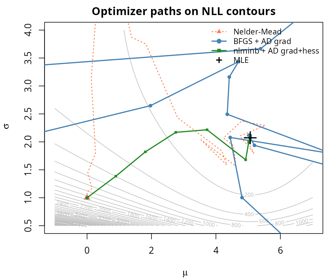

The Nelder-Mead simplex method (no derivatives) requires many more function evaluations and takes a wandering path. BFGS with the AD gradient converges more efficiently. nlminb() with both gradient and Hessian can achieve the most direct path to the optimum.

Summary

What you need	Function	R optimizer argument
Gradient	`gradient(f, x)`	`gr` in `optim()`, `gradient` in `nlminb()`
Hessian	`hessian(f, x)`	`hessian` in `nlminb()` only
Observed information	`-hessian(f, x)`	Post-optimization: invert for SEs

When to use which optimizer:

optim() with BFGS — good default; use gr = function(x) -gradient(f, x)
nlminb() — when you want second-order convergence; supply both gradient and Hessian
Nelder-Mead — fallback for non-smooth objectives; doesn’t benefit from AD

Remember the sign convention: optimizers minimize. For maximization, negate the function, gradient, and Hessian when passing to the optimizer.