Higher-Order Derivatives

library(nabla)
#> 
#> Attaching package: 'nabla'
#> The following objects are masked from 'package:stats':
#> 
#>     D, deriv

Nested duals

First-order duals give us $f(x)$ and $f'(x)$ . To also get $f''(x)$ , nabla uses nested duals — a dual number whose components are themselves dual numbers.

The structure dual(dual(x, 1), dual(1, 0)) simultaneously tracks:

$f(x)$ — the value of the inner value
$f'(x)$ — the derivative of the inner value
$f''(x)$ — the derivative of the outer derivative

x <- dual_variable_n(2, order = 2)

# Evaluate x^3
result <- x^3

# Extract all three quantities
deriv_n(result, 0)  # f(2) = 8
#> [1] 8
deriv_n(result, 1)  # f'(2) = 3*4 = 12
#> [1] 12
deriv_n(result, 2)  # f''(2) = 6*2 = 12
#> [1] 12

For constants in higher-order computations, use dual_constant_n():

k <- dual_constant_n(5, order = 2)
deriv_n(k, 0)  # 5
#> [1] 5
deriv_n(k, 1)  # 0
#> [1] 0
deriv_n(k, 2)  # 0
#> [1] 0

The `differentiate_n()` helper

For quick evaluation, differentiate_n() wraps the construction and extraction:

# Differentiate sin(x) at x = pi/4
result <- differentiate_n(sin, pi / 4, order = 2)
result$value   # sin(pi/4)
#> [1] 0.7071068
result$d1      # cos(pi/4) = f'
#> [1] 0.7071068
result$d2      # -sin(pi/4) = f''
#> [1] -0.7071068

Verify against known values:

result$value - sin(pi / 4)     # ~0
#> [1] 0
result$d1 - cos(pi / 4)        # ~0
#> [1] 0
result$d2 - (-sin(pi / 4))     # ~0
#> [1] 0

More complex functions work too:

f <- function(x) x * exp(-x^2)
d2 <- differentiate_n(f, 1, order = 2)

# Analytical: f'(x) = exp(-x^2)(1 - 2x^2)
# f''(x) = exp(-x^2)(-6x + 4x^3)
analytical_f1 <- exp(-1) * (1 - 2)
analytical_f2 <- exp(-1) * (-6 + 4)
d2$d1 - analytical_f1   # ~0
#> [1] 0
d2$d2 - analytical_f2   # ~0
#> [1] 0

The `D` operator

The D operator provides a composable way to compute derivatives of multi-parameter functions. D(f) returns the derivative of f as a new function, and compositions D(D(f)) yield higher-order derivative tensors:

# Gradient of a 2-parameter function
f <- function(x) x[1]^2 * x[2]
D(f, c(3, 4))  # gradient: c(24, 9)
#> [1] 24  9

# Hessian via D^2
D(f, c(3, 4), order = 2)
#>      [,1] [,2]
#> [1,]    8    6
#> [2,]    6    0

# Composition works identically
Df <- D(f)
DDf <- D(Df)
DDf(c(3, 4))
#>      [,1] [,2]
#> [1,]    8    6
#> [2,]    6    0

For vector-valued functions, D produces the Jacobian:

g <- function(x) list(x[1] * x[2], x[1]^2 + x[2])
D(g, c(3, 4))  # 2x2 Jacobian: [[4, 3], [6, 1]]
#>      [,1] [,2]
#> [1,]    4    3
#> [2,]    6    1

The convenience functions gradient(), hessian(), and jacobian() are thin wrappers around D:

gradient(f, c(3, 4))           # == D(f, c(3, 4))
#> [1] 24  9
hessian(f, c(3, 4))            # == D(f, c(3, 4), order = 2)
#>      [,1] [,2]
#> [1,]    8    6
#> [2,]    6    0
jacobian(g, c(3, 4))           # == D(g, c(3, 4))
#>      [,1] [,2]
#> [1,]    4    3
#> [2,]    6    1

Curvature analysis

The curvature of a curve $y = f(x)$ is:

$\kappa = \frac{|f''(x)|}{(1 + f'(x)^2)^{3/2}}$

With second-order AD, we can compute this directly:

curvature <- function(f, x) {
  d2 <- differentiate_n(f, x, order = 2)
  abs(d2$d2) / (1 + d2$d1^2)^(3/2)
}

# Curvature of sin(x) at various points
xs <- seq(0, 2 * pi, length.out = 7)
kappas <- sapply(xs, function(x) curvature(sin, x))
data.frame(x = round(xs, 3), curvature = round(kappas, 6))
#>       x curvature
#> 1 0.000  0.000000
#> 2 1.047  0.619677
#> 3 2.094  0.619677
#> 4 3.142  0.000000
#> 5 4.189  0.619677
#> 6 5.236  0.619677
#> 7 6.283  0.000000

The pattern in the table reveals the geometry of $\sin(x)$ : curvature is zero at the inflection points (integer multiples of $\pi$ , where $\sin''(x) = 0$ ), and peaks at $\pi/2$ and $3\pi/2$ where $\sin$ reaches its extreme values. The maximum curvature of 1.0 occurs because $\sin$ has unit amplitude — for $A\sin(x)$ the maximum curvature would be $A$ .

At $x = \pi/2$ , $\sin$ has maximum curvature because $|\sin''(\pi/2)| = 1$ and $\sin'(\pi/2) = 0$ :

curvature(sin, pi / 2)  # should be 1.0
#> [1] 1

Visualizing curvature along sin(x)

Curvature peaks where the second derivative is largest in magnitude and the first derivative is small. For $\sin(x)$ , this occurs at $\pi/2$ and $3\pi/2$ :

xs_curve <- seq(0, 2 * pi, length.out = 200)
sin_vals <- sin(xs_curve)
kappa_vals <- sapply(xs_curve, function(x) curvature(sin, x))

par(mar = c(4, 4.5, 2, 4.5))
plot(xs_curve, sin_vals, type = "l", col = "steelblue", lwd = 2,
     xlab = "x", ylab = "sin(x)",
     main = "sin(x) and its curvature")
par(new = TRUE)
plot(xs_curve, kappa_vals, type = "l", col = "firebrick", lwd = 2, lty = 2,
     axes = FALSE, xlab = "", ylab = "")
axis(4, col.axis = "firebrick")
mtext(expression(kappa(x)), side = 4, line = 2.5, col = "firebrick")
abline(v = c(pi / 2, 3 * pi / 2), col = "grey60", lty = 3)
legend("bottom",
       legend = c("sin(x)", expression(kappa(x))),
       col = c("steelblue", "firebrick"), lty = c(1, 2), lwd = 2,
       bty = "n", horiz = TRUE)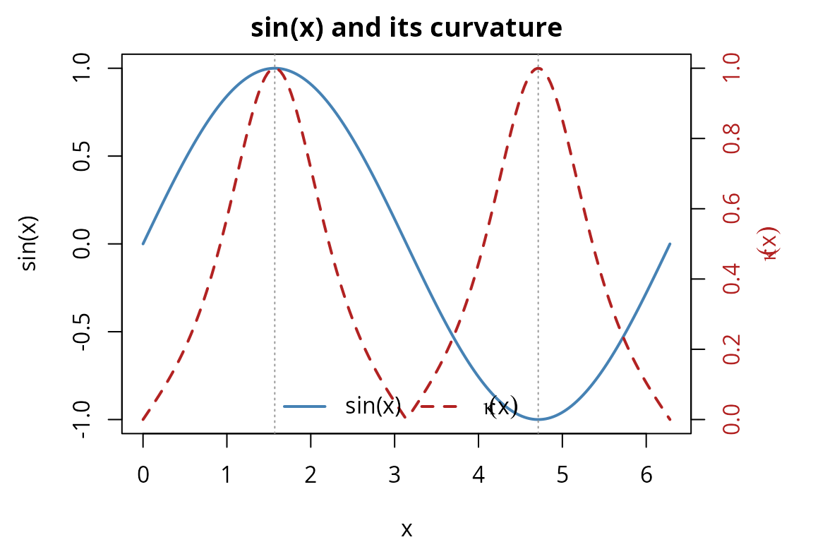

The curvature reaches its maximum of 1.0 at $x = \pi/2$ (where $\sin'(x) = 0$ and $|\sin''(x)| = 1$ ) and returns to zero at integer multiples of $\pi$ (where $\sin''(x) = 0$ ).

Taylor expansion

A second-order Taylor approximation of $f$ around $x_0$ :

$f(x) \approx f(x_0) + f'(x_0)(x - x_0) + \frac{1}{2} f''(x_0)(x - x_0)^2$

We can compute this using nested duals:

taylor2 <- function(f, x0, x) {
  d2 <- differentiate_n(f, x0, order = 2)
  d2$value + d2$d1 * (x - x0) + 0.5 * d2$d2 * (x - x0)^2
}

# Approximate exp(x) near x = 0
f_exp <- function(x) exp(x)
xs <- c(-0.1, -0.01, 0, 0.01, 0.1)
data.frame(
  x = xs,
  exact = exp(xs),
  taylor2 = sapply(xs, function(x) taylor2(f_exp, 0, x)),
  error = exp(xs) - sapply(xs, function(x) taylor2(f_exp, 0, x))
)
#>       x     exact taylor2         error
#> 1 -0.10 0.9048374 0.90500 -1.625820e-04
#> 2 -0.01 0.9900498 0.99005 -1.662508e-07
#> 3  0.00 1.0000000 1.00000  0.000000e+00
#> 4  0.01 1.0100502 1.01005  1.670842e-07
#> 5  0.10 1.1051709 1.10500  1.709181e-04

Near the expansion point, the approximation is very accurate. The error grows as $O(|x - x_0|^3)$ because the Taylor remainder is $\frac{f'''(\xi)}{6}(x - x_0)^3$ . For $\exp(x)$ around $x_0 = 0$ , $f'''(\xi) = \exp(\xi) \approx 1$ , so the error at $x = 0.1$ is approximately $0.1^3/6 \approx 1.7 \times 10^{-4}$ and at $x = 0.01$ it drops to $\approx 1.7 \times 10^{-7}$ — a factor-of-1000 reduction for a factor-of-10 decrease in distance, confirming cubic convergence. We can see this divergence visually:

xs_plot <- seq(-2, 3, length.out = 300)
exact_vals <- exp(xs_plot)
taylor_vals <- sapply(xs_plot, function(x) taylor2(f_exp, 0, x))

par(mar = c(4, 4, 2, 1))
plot(xs_plot, exact_vals, type = "l", col = "steelblue", lwd = 2,
     xlab = "x", ylab = "y",
     main = expression("exp(x) vs 2nd-order Taylor at " * x[0] == 0),
     ylim = c(-1, 12))
lines(xs_plot, taylor_vals, col = "firebrick", lwd = 2, lty = 2)
abline(v = 0, col = "grey60", lty = 3)
points(0, 1, pch = 19, col = "grey40", cex = 1.2)
legend("topleft",
       legend = c("exp(x)", expression("Taylor " * T[2](x))),
       col = c("steelblue", "firebrick"), lty = c(1, 2), lwd = 2,
       bty = "n")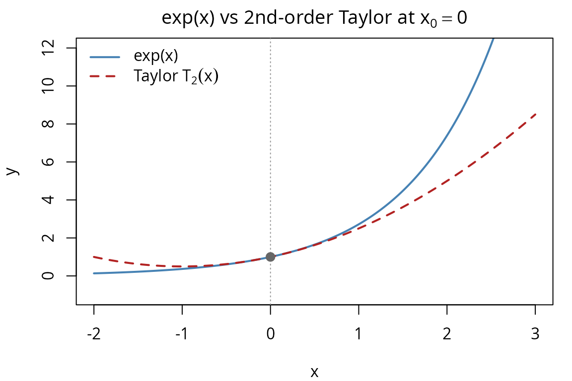

The Taylor polynomial matches exp(x) closely near $x_0 = 0$ but diverges at larger distances, illustrating the local nature of polynomial approximation.

Connection to MLE: Hessian via nested duals

The hessian() function in nabla uses the D operator internally. We can verify this by manually constructing a second-order dual for a log-likelihood and comparing with the hessian() helper.

Consider a Poisson log-likelihood for $\lambda$ :

set.seed(123)
data_pois <- rpois(50, lambda = 3)
n <- length(data_pois)
sum_x <- sum(data_pois)
sum_lfact <- sum(lfactorial(data_pois))

ll_poisson <- function(theta) {
  lambda <- theta[1]
  sum_x * log(lambda) - n * lambda - sum_lfact
}

lambda0 <- 2.5

Method 1: Using hessian() helper:

hess_helper <- hessian(ll_poisson, lambda0)
hess_helper
#>       [,1]
#> [1,] -24.8

Method 2: Manual nested dual construction:

# Build a dual_variable_n wrapped in a dual_vector
manual_theta <- dual_vector(list(dual_variable_n(lambda0, 2)))
result_manual <- ll_poisson(manual_theta)
manual_hess <- deriv(deriv(result_manual))
manual_hess
#> [1] -24.8

Both approaches yield the same result:

hess_helper[1, 1] - manual_hess  # ~0
#> [1] 0

This shows that hessian() is simply an organized wrapper around the same nested dual arithmetic.

Summary

Nested dual numbers extend forward-mode AD to second derivatives in a single forward pass — no symbolic differentiation, no finite-difference grid, and no loss of precision:

Exact second derivatives. By nesting $\varepsilon_1$ inside $\varepsilon_2$ , every arithmetic operation simultaneously propagates $f(x)$ , $f'(x)$ , and $f''(x)$ .
This is the engine behind hessian(). The convenience function hessian() constructs nested duals internally for each parameter pair and extracts the second-derivative matrix — the same arithmetic shown in the manual construction above.
Practical applications. Curvature analysis, Taylor approximation, and Newton-Raphson optimization all depend on accurate second derivatives. Nested duals provide these without the step-size tuning that plagues numerical second differences.