Introduction to nabla • nabla

library(nabla)
#> 
#> Attaching package: 'nabla'
#> The following objects are masked from 'package:stats':
#> 
#>     D, deriv

What are dual numbers?

A dual number has the form $a + b\varepsilon$ , where $\varepsilon$ is an abstract quantity satisfying $\varepsilon^2 = 0$ . This seemingly simple idea gives us exact first derivatives for free.

When we evaluate a function $f$ on a dual number $x + \varepsilon$ :

$f(x + \varepsilon) = f(x) + f'(x)\,\varepsilon$

The “value” part gives $f(x)$ and the “epsilon” part gives $f'(x)$ , computed automatically by propagating $\varepsilon$ through every arithmetic operation. This is forward-mode automatic differentiation (AD) — no symbolic algebra, no finite differences, just exact derivatives at machine precision.

Basic usage

Create dual numbers with dual(), or use the convenience constructors:

# A dual variable: value = 3, derivative seed = 1
x <- dual_variable(3)
value(x)
#> [1] 3
deriv(x)
#> [1] 1

# A dual constant: value = 5, derivative seed = 0
k <- dual_constant(5)
value(k)
#> [1] 5
deriv(k)
#> [1] 0

# Explicit constructor
y <- dual(2, 1)
value(y)
#> [1] 2
deriv(y)
#> [1] 1

Setting deriv = 1 means “I’m differentiating with respect to this variable.” Setting deriv = 0 means “this is a constant.”

Arithmetic

All standard arithmetic operators propagate derivatives:

x <- dual_variable(3)

# Addition: d/dx(x + 2) = 1
r_add <- x + 2
value(r_add)
#> [1] 5
deriv(r_add)
#> [1] 1

# Subtraction: d/dx(5 - x) = -1
r_sub <- 5 - x
value(r_sub)
#> [1] 2
deriv(r_sub)
#> [1] -1

# Multiplication: d/dx(x * 4) = 4
r_mul <- x * 4
value(r_mul)
#> [1] 12
deriv(r_mul)
#> [1] 4

# Division: d/dx(1/x) = -1/x^2 = -1/9
r_div <- 1 / x
value(r_div)
#> [1] 0.3333333
deriv(r_div)
#> [1] -0.1111111

# Power: d/dx(x^3) = 3*x^2 = 27
r_pow <- x^3
value(r_pow)
#> [1] 27
deriv(r_pow)
#> [1] 27

Math functions

All standard mathematical functions are supported, with derivatives computed via the chain rule:

x <- dual_variable(1)

# exp: d/dx exp(x) = exp(x)
r_exp <- exp(x)
value(r_exp)
#> [1] 2.718282
deriv(r_exp)
#> [1] 2.718282

# log: d/dx log(x) = 1/x
r_log <- log(x)
value(r_log)
#> [1] 0
deriv(r_log)
#> [1] 1

# sin: d/dx sin(x) = cos(x)
x2 <- dual_variable(pi / 4)
r_sin <- sin(x2)
value(r_sin)
#> [1] 0.7071068
deriv(r_sin)  # cos(pi/4)
#> [1] 0.7071068

# sqrt: d/dx sqrt(x) = 1/(2*sqrt(x))
x3 <- dual_variable(4)
r_sqrt <- sqrt(x3)
value(r_sqrt)
#> [1] 2
deriv(r_sqrt)  # 1/(2*2) = 0.25
#> [1] 0.25

# Gamma-related
x4 <- dual_variable(3)
r_lgamma <- lgamma(x4)
value(r_lgamma)     # log(2!) = log(2)
#> [1] 0.6931472
deriv(r_lgamma)     # digamma(3)
#> [1] 0.9227843

Composition

User-defined functions “just work” — no special annotation needed:

f <- function(x) x^2 + sin(x)

# Evaluate at pi/4
x <- dual_variable(pi / 4)
result <- f(x)
value(result)   # (pi/4)^2 + sin(pi/4)
#> [1] 1.323957
deriv(result)   # 2*(pi/4) + cos(pi/4)
#> [1] 2.277903

# Verify
analytical <- 2 * (pi / 4) + cos(pi / 4)
deriv(result) - analytical  # ~0
#> [1] 0

We can visualize both a function and its AD-computed derivative over an interval. Here we plot $f(x) = x^2 + \sin(x)$ and $f'(x) = 2x + \cos(x)$ over $[0, 2\pi]$ , marking the evaluation point $x = \pi/4$ :

f <- function(x) x^2 + sin(x)
xs <- seq(0, 2 * pi, length.out = 200)

# Compute f(x) and f'(x) at each grid point using AD
vals <- sapply(xs, function(xi) {
  r <- f(dual_variable(xi))
  c(value(r), deriv(r))
})
fx <- vals[1, ]
fpx <- vals[2, ]

# Mark the evaluation point x = pi/4
x_mark <- pi / 4
r_mark <- f(dual_variable(x_mark))

par(mar = c(4, 4, 2, 1))
plot(xs, fx, type = "l", col = "steelblue", lwd = 2,
     xlab = "x", ylab = "y",
     main = expression(f(x) == x^2 + sin(x) ~ "and its derivative"),
     ylim = range(c(fx, fpx)))
lines(xs, fpx, col = "firebrick", lwd = 2, lty = 2)
points(x_mark, value(r_mark), pch = 19, col = "steelblue", cex = 1.3)
points(x_mark, deriv(r_mark), pch = 19, col = "firebrick", cex = 1.3)
abline(v = x_mark, col = "grey60", lty = 3)
legend("topleft", legend = c("f(x)", "f'(x) via AD"),
       col = c("steelblue", "firebrick"), lty = c(1, 2), lwd = 2,
       bty = "n")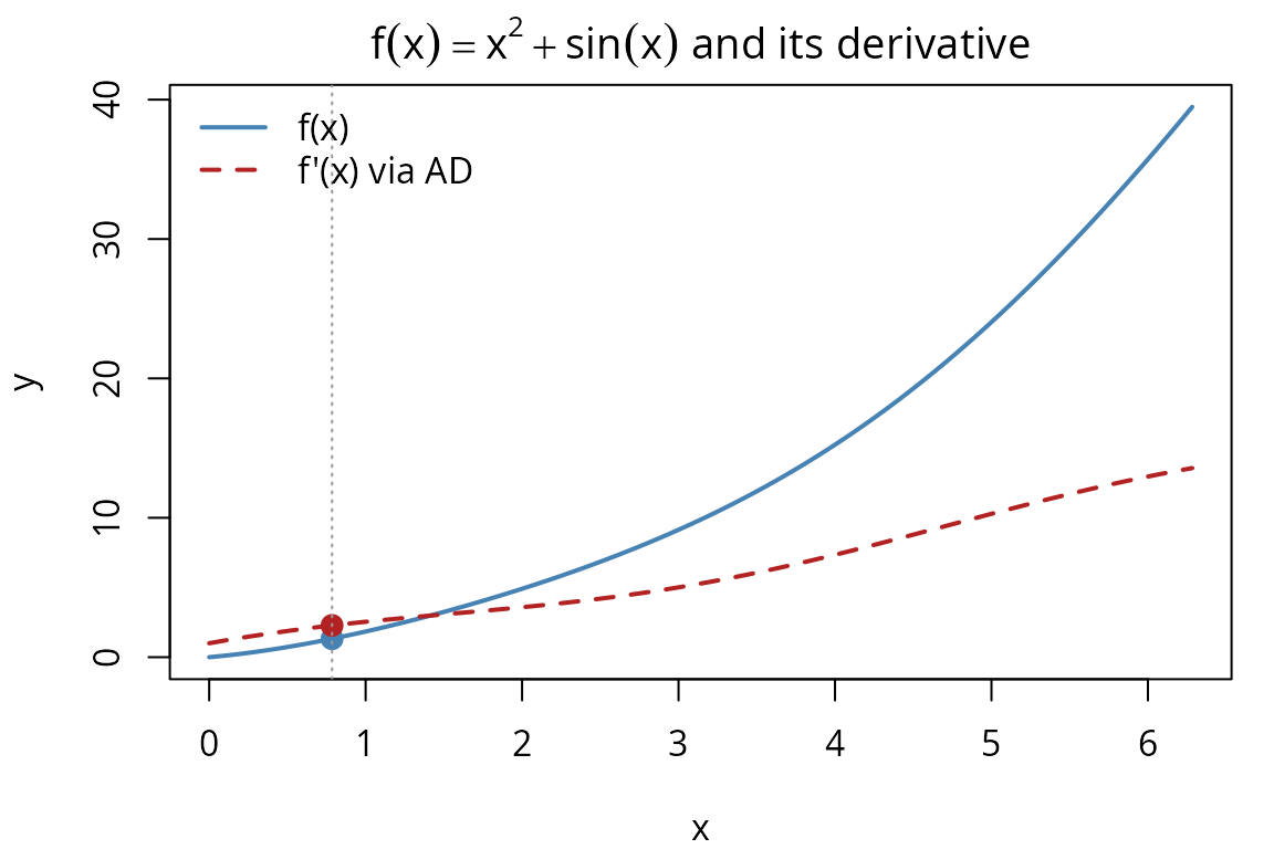

More complex compositions also propagate correctly:

g <- function(x) exp(-x^2 / 2) / sqrt(2 * pi)  # standard normal PDF

x <- dual_variable(1)
result <- g(x)
value(result)   # dnorm(1)
#> [1] 0.2419707
# derivative: -x * dnorm(x)
analytical <- -1 * dnorm(1)
deriv(result) - analytical  # ~0
#> [1] 0

Base R interop

Dual numbers integrate with standard R patterns:

# sum() works
a <- dual_variable(2)
b <- dual_constant(3)
total <- sum(a, b, dual_constant(1))
value(total)  # 6
#> [1] 6
deriv(total)  # 1 (only a has deriv = 1)
#> [1] 1

# prod() works
p <- prod(a, dual_constant(3))
value(p)  # 6
#> [1] 6
deriv(p)  # 3 (product rule: 3*1 + 2*0)
#> [1] 3

# c() creates a dual_vector
v <- c(a, b)
length(v)
#> [1] 2

# is.numeric returns TRUE (for compatibility)
is.numeric(dual_variable(1))
#> [1] TRUE

Control flow and iteration work naturally:

# if/else branching
safe_log <- function(x) {
  if (x > 0) log(x) else dual_constant(-Inf)
}
value(safe_log(dual_variable(2)))
#> [1] 0.6931472
deriv(safe_log(dual_variable(2)))
#> [1] 0.5

# for loop
x <- dual_variable(2)
accum <- dual_constant(0)
for (i in 1:5) {
  accum <- accum + x^i
}
value(accum)  # 2 + 4 + 8 + 16 + 32 = 62
#> [1] 62
deriv(accum)  # 1 + 4 + 12 + 32 + 80 = 129
#> [1] 129

# Reduce
terms <- list(dual_variable(2), dual_constant(3), dual_constant(4))
total <- Reduce("+", terms)
value(total)
#> [1] 9
deriv(total)
#> [1] 1

# sapply (extract values)
vals <- c(dual_variable(1), dual_constant(2), dual_constant(3))
sapply(seq_along(vals@.Data), function(i) value(vals[[i]]))
#> [1] 1 2 3

Quick comparison: three ways to differentiate

Let’s compare three methods of computing the derivative of $f(x) = x^3 \sin(x)$ at $x = 2$ :

f <- function(x) x^3 * sin(x)

x0 <- 2

# 1. Analytical: f'(x) = 3x^2 sin(x) + x^3 cos(x)
analytical <- 3 * x0^2 * sin(x0) + x0^3 * cos(x0)

# 2. Finite differences
h <- 1e-8
finite_diff <- (f(x0 + h) - f(x0 - h)) / (2 * h)

# 3. Automatic differentiation
ad_result <- deriv(f(dual_variable(x0)))

# Compare
data.frame(
  method = c("Analytical", "Finite Diff", "AD (nabla)"),
  derivative = c(analytical, finite_diff, ad_result),
  error_vs_analytical = c(0, finite_diff - analytical, ad_result - analytical)
)
#>        method derivative error_vs_analytical
#> 1  Analytical   7.582394         0.00000e+00
#> 2 Finite Diff   7.582394        -1.17109e-07
#> 3  AD (nabla)   7.582394         0.00000e+00

The AD result matches the analytical derivative to machine precision — zero error — because dual-number arithmetic propagates exact derivative rules through every operation. Finite differences, by contrast, introduce truncation error of order $O(h^2)$ for central differences; here the error is roughly $10^{-7}$ , reflecting the choice of $h = 10^{-8}$ (the optimal step size for double-precision central differences is approximately $\epsilon_{\mathrm{mach}}^{1/3} \approx 6 \times 10^{-6}$ , so our step is in the right ballpark). A bar chart makes this difference vivid:

errors <- abs(c(finite_diff - analytical, ad_result - analytical))
# Use log10 scale; clamp AD error to .Machine$double.eps if exactly zero
errors[errors == 0] <- .Machine$double.eps

par(mar = c(4, 5, 2, 1))
bp <- barplot(log10(errors),
              names.arg = c("Finite Diff", "AD (nabla)"),
              col = c("coral", "steelblue"),
              ylab = expression(log[10] ~ "|error|"),
              main = "Absolute error vs analytical derivative",
              ylim = c(-16, 0), border = NA)
abline(h = log10(.Machine$double.eps), lty = 2, col = "grey40")
text(mean(bp), log10(.Machine$double.eps) + 0.8,
     "machine epsilon", cex = 0.8, col = "grey40")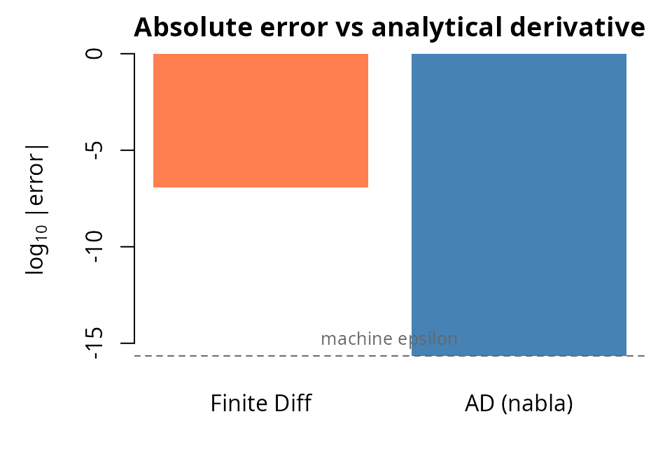

This advantage becomes critical for optimization algorithms that depend on accurate gradients.

What’s next?

This vignette covered the fundamentals of dual-number arithmetic and showed that AD computes exact derivatives where finite differences cannot. To see how this pays off in practice:

vignette("mle-workflow") applies score(), hessian(), and observed_information() to five increasingly complex MLE problems, from Normal to logistic regression, and builds a Newton-Raphson optimizer powered entirely by AD.
vignette("higher-order") demonstrates nested duals for second derivatives, with applications to curvature analysis and Taylor expansion.
vignette("optimizer-integration") shows how to plug nabla gradients into R’s built-in optimizers (optim, nlminb) for production-quality MLE fitting.