Gradient and Hessian Computation with nabla

library(nabla)
#> 
#> Attaching package: 'nabla'
#> The following objects are masked from 'package:stats':
#> 
#>     D, deriv

This vignette demonstrates nabla’s gradient() and hessian() functions on several functions. For each, we compare derivatives computed three ways:

Analytical — hand-derived formulas
Finite differences — numerical approximation
AD (nabla) — automatic differentiation via gradient() and hessian()

Helper: finite difference utilities

We’ll use central differences for numerical comparison:

numerical_gradient <- function(f, x, h = 1e-7) {
  p <- length(x)
  grad <- numeric(p)
  for (i in seq_len(p)) {
    x_plus <- x_minus <- x
    x_plus[i] <- x[i] + h
    x_minus[i] <- x[i] - h
    grad[i] <- (f(x_plus) - f(x_minus)) / (2 * h)
  }
  grad
}

numerical_hessian <- function(f, x, h = 1e-5) {
  p <- length(x)
  H <- matrix(0, nrow = p, ncol = p)
  for (i in seq_len(p)) {
    for (j in seq_len(i)) {
      x_pp <- x_pm <- x_mp <- x_mm <- x
      x_pp[i] <- x_pp[i] + h; x_pp[j] <- x_pp[j] + h
      x_pm[i] <- x_pm[i] + h; x_pm[j] <- x_pm[j] - h
      x_mp[i] <- x_mp[i] - h; x_mp[j] <- x_mp[j] + h
      x_mm[i] <- x_mm[i] - h; x_mm[j] <- x_mm[j] - h
      H[i, j] <- (f(x_pp) - f(x_pm) - f(x_mp) + f(x_mm)) / (4 * h * h)
      H[j, i] <- H[i, j]
    }
  }
  H
}

Normal log-likelihood: known sigma, unknown mu

A simple starting example. Given data $x_1, \ldots, x_n$ with known $\sigma$ , the log-likelihood for $\mu$ is:

$\ell(\mu) = -\frac{1}{2\sigma^2} \sum_{i=1}^n (x_i - \mu)^2 + \text{const}$

Using sufficient statistics ( $\bar{x}$ , $n$ ), this simplifies.

set.seed(42)
data_norm <- rnorm(100, mean = 5, sd = 2)
n <- length(data_norm)
sigma <- 2
sum_x <- sum(data_norm)
sum_x2 <- sum(data_norm^2)

ll_normal_mu <- function(x) {
  mu <- x[1]
  -1 / (2 * sigma^2) * (sum_x2 - 2 * mu * sum_x + n * mu^2)
}

# Evaluate at mu = 4.5
mu0 <- 4.5

# AD gradient and Hessian
ad_grad <- gradient(ll_normal_mu, mu0)
ad_hess <- hessian(ll_normal_mu, mu0)

# Analytical: gradient = (sum_x - n*mu)/sigma^2, Hessian = -n/sigma^2
xbar <- mean(data_norm)
analytical_grad <- (sum_x - n * mu0) / sigma^2
analytical_hess <- -n / sigma^2

# Numerical
num_grad <- numerical_gradient(ll_normal_mu, mu0)
num_hess <- numerical_hessian(ll_normal_mu, mu0)

# Three-way comparison: Gradient
data.frame(
  method = c("Analytical", "Finite Diff", "AD"),
  gradient = c(analytical_grad, num_grad, ad_grad)
)
#>        method gradient
#> 1  Analytical 14.12574
#> 2 Finite Diff 14.12574
#> 3          AD 14.12574

# Three-way comparison: Hessian
data.frame(
  method = c("Analytical", "Finite Diff", "AD"),
  hessian = c(analytical_hess, num_hess, ad_hess)
)
#>        method   hessian
#> 1  Analytical -25.00000
#> 2 Finite Diff -24.99974
#> 3          AD -25.00000

All three methods agree to machine precision for this simple quadratic function. The gradient is linear in $\mu$ and the Hessian is constant ( $-n/\sigma^2 = -25$ ), so there are no higher-order terms for finite differences to approximate poorly. This serves as a sanity check that the AD machinery is wired correctly.

The observed information (negative Hessian) is simply:

obs_info <- -hessian(ll_normal_mu, mu0)
obs_info  # should equal n/sigma^2 = 25
#>      [,1]
#> [1,]   25

Normal log-likelihood: unknown mu and sigma

Now both $\mu$ and $\sigma$ are unknown. The log-likelihood is:

$\ell(\mu, \sigma) = -n \log(\sigma) - \frac{1}{2\sigma^2}\sum(x_i - \mu)^2$

ll_normal_2 <- function(x) {
  mu <- x[1]
  sigma <- x[2]
  -n * log(sigma) - (1 / (2 * sigma^2)) * (sum_x2 - 2 * mu * sum_x + n * mu^2)
}

theta0 <- c(4.5, 1.8)

# AD
ad_grad2 <- gradient(ll_normal_2, theta0)
ad_hess2 <- hessian(ll_normal_2, theta0)

# Analytical gradient:
# d/dmu = n*(xbar - mu)/sigma^2
# d/dsigma = -n/sigma + (1/sigma^3)*sum((xi - mu)^2)
mu0_2 <- theta0[1]; sigma0_2 <- theta0[2]
ss <- sum_x2 - 2 * mu0_2 * sum_x + n * mu0_2^2  # sum of (xi - mu)^2
analytical_grad2 <- c(
  n * (xbar - mu0_2) / sigma0_2^2,
  -n / sigma0_2 + ss / sigma0_2^3
)

# Analytical Hessian:
# d2/dmu2 = -n/sigma^2
# d2/dsigma2 = n/sigma^2 - 3*ss/sigma^4
# d2/dmu.dsigma = -2*n*(xbar - mu)/sigma^3
analytical_hess2 <- matrix(c(
  -n / sigma0_2^2,
  -2 * n * (xbar - mu0_2) / sigma0_2^3,
  -2 * n * (xbar - mu0_2) / sigma0_2^3,
  n / sigma0_2^2 - 3 * ss / sigma0_2^4
), nrow = 2, byrow = TRUE)

# Numerical
num_grad2 <- numerical_gradient(ll_normal_2, theta0)
num_hess2 <- numerical_hessian(ll_normal_2, theta0)

# Gradient comparison
data.frame(
  parameter = c("mu", "sigma"),
  analytical = analytical_grad2,
  finite_diff = num_grad2,
  AD = ad_grad2
)
#>   parameter analytical finite_diff       AD
#> 1        mu   17.43919    17.43919 17.43919
#> 2     sigma   23.55245    23.55245 23.55245

# Hessian comparison (flatten for display)
cat("AD Hessian:\n")
#> AD Hessian:
ad_hess2
#>           [,1]       [,2]
#> [1,] -30.86420  -19.37687
#> [2,] -19.37687 -100.98248
cat("\nAnalytical Hessian:\n")
#> 
#> Analytical Hessian:
analytical_hess2
#>           [,1]       [,2]
#> [1,] -30.86420  -19.37687
#> [2,] -19.37687 -100.98248
cat("\nMax absolute difference:", max(abs(ad_hess2 - analytical_hess2)), "\n")
#> 
#> Max absolute difference: 2.842171e-14

The maximum absolute difference between the AD and analytical Hessians is at the level of machine epsilon ( $\sim 10^{-14}$ ), confirming that AD computes exact second derivatives even for this two-parameter model. The cross-derivative $\partial^2 \ell / \partial\mu\,\partial\sigma$ is non-zero when $\mu \ne \bar{x}$ , exercising the mixed-partial logic in nested dual arithmetic.

Poisson log-likelihood: unknown lambda

Given count data $x_1, \ldots, x_n$ from Poisson( $\lambda$ ):

$\ell(\lambda) = \bar{x} \cdot n \log(\lambda) - n\lambda - \sum \log(x_i!)$

set.seed(123)
data_pois <- rpois(80, lambda = 3.5)
n_pois <- length(data_pois)
sum_x_pois <- sum(data_pois)
sum_lfact <- sum(lfactorial(data_pois))

ll_poisson <- function(x) {
  lambda <- x[1]
  sum_x_pois * log(lambda) - n_pois * lambda - sum_lfact
}

lam0 <- 3.0

# AD
ad_grad_p <- gradient(ll_poisson, lam0)
ad_hess_p <- hessian(ll_poisson, lam0)

# Analytical: gradient = sum_x/lambda - n, Hessian = -sum_x/lambda^2
analytical_grad_p <- sum_x_pois / lam0 - n_pois
analytical_hess_p <- -sum_x_pois / lam0^2

# Numerical
num_grad_p <- numerical_gradient(ll_poisson, lam0)
num_hess_p <- numerical_hessian(ll_poisson, lam0)

data.frame(
  quantity = c("Gradient", "Hessian"),
  analytical = c(analytical_grad_p, analytical_hess_p),
  finite_diff = c(num_grad_p, num_hess_p),
  AD = c(ad_grad_p, ad_hess_p)
)
#>   quantity analytical finite_diff        AD
#> 1 Gradient   13.66667    13.66667  13.66667
#> 2  Hessian  -31.22222   -31.22238 -31.22222

Again, all three methods agree exactly. The Poisson log-likelihood involves only log(lambda) and linear terms in $\lambda$ , so the sufficient statistics produce clean rational expressions for the gradient and Hessian — making this an ideal test case for verifying AD correctness.

Visualizing the gradient

The gradient of a function is zero at its optimum. We can see this by plotting the log-likelihood and its gradient together:

lam_grid <- seq(2.0, 5.5, length.out = 200)

# Compute log-likelihood and gradient over the grid
ll_vals <- sapply(lam_grid, function(l) ll_poisson(l))
gr_vals <- sapply(lam_grid, function(l) gradient(ll_poisson, l))

mle_lam <- sum_x_pois / n_pois  # analytical MLE

par(mar = c(4, 4.5, 2, 4.5))
plot(lam_grid, ll_vals, type = "l", col = "steelblue", lwd = 2,
     xlab = expression(lambda), ylab = expression(ell(lambda)),
     main = "Poisson log-likelihood and gradient")
par(new = TRUE)
plot(lam_grid, gr_vals, type = "l", col = "firebrick", lwd = 2, lty = 2,
     axes = FALSE, xlab = "", ylab = "")
axis(4, col.axis = "firebrick")
mtext("Gradient", side = 4, line = 2.5, col = "firebrick")
abline(h = 0, col = "grey60", lty = 3)
abline(v = mle_lam, col = "grey40", lty = 3)
points(mle_lam, 0, pch = 4, col = "firebrick", cex = 1.5, lwd = 2)
legend("topright",
       legend = c(expression(ell(lambda)), "Gradient", "MLE"),
       col = c("steelblue", "firebrick", "grey40"),
       lty = c(1, 2, 3), lwd = c(2, 2, 1), pch = c(NA, NA, 4),
       bty = "n")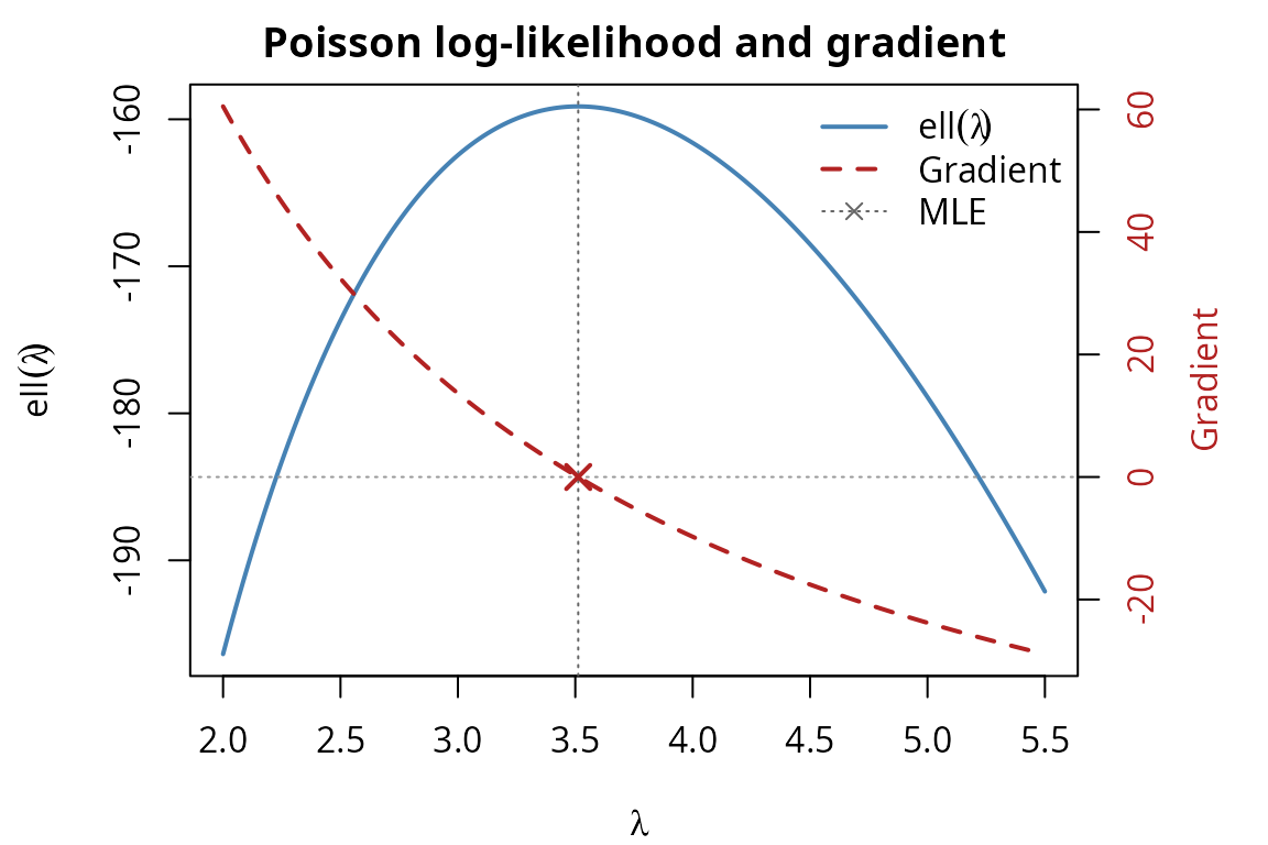

The gradient crosses zero exactly at the MLE ( $\hat\lambda = \bar{x}$ ), confirming that our AD-computed gradient is consistent with the analytical solution.

Gamma log-likelihood: unknown shape, known rate

The Gamma distribution with shape $\alpha$ and known rate $\beta = 1$ has log-likelihood:

$\ell(\alpha) = (\alpha - 1)\sum \log x_i - n\log\Gamma(\alpha) + n\alpha\log(\beta) - \beta\sum x_i$

This is interesting because it involves lgamma and digamma.

set.seed(99)
data_gamma <- rgamma(60, shape = 2.5, rate = 1)
n_gam <- length(data_gamma)
sum_log_x <- sum(log(data_gamma))
sum_x_gam <- sum(data_gamma)
beta_known <- 1

ll_gamma <- function(x) {
  alpha <- x[1]
  (alpha - 1) * sum_log_x - n_gam * lgamma(alpha) +
    n_gam * alpha * log(beta_known) - beta_known * sum_x_gam
}

alpha0 <- 2.0

# AD
ad_grad_g <- gradient(ll_gamma, alpha0)
ad_hess_g <- hessian(ll_gamma, alpha0)

# Analytical: gradient = sum_log_x - n*digamma(alpha) + n*log(beta)
# Hessian = -n*trigamma(alpha)
analytical_grad_g <- sum_log_x - n_gam * digamma(alpha0) + n_gam * log(beta_known)
analytical_hess_g <- -n_gam * trigamma(alpha0)

# Numerical
num_grad_g <- numerical_gradient(ll_gamma, alpha0)
num_hess_g <- numerical_hessian(ll_gamma, alpha0)

data.frame(
  quantity = c("Gradient", "Hessian"),
  analytical = c(analytical_grad_g, analytical_hess_g),
  finite_diff = c(num_grad_g, num_hess_g),
  AD = c(ad_grad_g, ad_hess_g)
)
#>   quantity analytical finite_diff        AD
#> 1 Gradient   16.97943    16.97943  16.97943
#> 2  Hessian  -38.69604   -38.69602 -38.69604

The Gamma model is a key differentiator between AD and finite differences. The log-likelihood involves lgamma(alpha), whose derivatives are digamma and trigamma — special functions that nabla propagates exactly through the chain rule. With finite differences, choosing a good step size $h$ for lgamma is tricky: too large introduces truncation error in the rapidly-varying digamma function, too small amplifies round-off. AD sidesteps this entirely by computing the exact digamma and trigamma values at each evaluation point.

Logistic regression: 2 predictors

For a binary response $y_i \in \{0, 1\}$ with design matrix $X$ and coefficients $\beta$ :

$\ell(\beta) = \sum_{i=1}^n \bigl[y_i \eta_i - \log(1 + e^{\eta_i})\bigr], \quad \eta_i = X_i \beta$

set.seed(7)
n_lr <- 50
X <- cbind(1, rnorm(n_lr), rnorm(n_lr))  # intercept + 2 predictors
beta_true <- c(-0.5, 1.2, -0.8)
eta_true <- X %*% beta_true
prob_true <- 1 / (1 + exp(-eta_true))
y <- rbinom(n_lr, 1, prob_true)

ll_logistic <- function(x) {
  result <- dual_constant(0)
  for (i in seq_len(n_lr)) {
    eta_i <- x[1] * X[i, 1] + x[2] * X[i, 2] + x[3] * X[i, 3]
    result <- result + y[i] * eta_i - log(1 + exp(eta_i))
  }
  result
}

beta0 <- c(0, 0, 0)

# AD
ad_grad_lr <- gradient(ll_logistic, beta0)
ad_hess_lr <- hessian(ll_logistic, beta0)

# Numerical
ll_logistic_num <- function(beta) {
  eta <- X %*% beta
  sum(y * eta - log(1 + exp(eta)))
}
num_grad_lr <- numerical_gradient(ll_logistic_num, beta0)
num_hess_lr <- numerical_hessian(ll_logistic_num, beta0)

# Gradient comparison
data.frame(
  parameter = c("beta0", "beta1", "beta2"),
  finite_diff = num_grad_lr,
  AD = ad_grad_lr,
  difference = ad_grad_lr - num_grad_lr
)
#>   parameter finite_diff        AD    difference
#> 1     beta0    -2.00000  -2.00000 -1.215494e-08
#> 2     beta1    11.10628  11.10628 -7.302688e-09
#> 3     beta2   -10.28118 -10.28118  2.067073e-08

# Hessian comparison
cat("Max |AD - numerical| in Hessian:", max(abs(ad_hess_lr - num_hess_lr)), "\n")
#> Max |AD - numerical| in Hessian: 2.56111e-05

The numerical Hessian difference ( $\sim 10^{-5}$ ) is noticeably larger than in the earlier models. This is because the logistic log-likelihood is computed via a loop over $n = 50$ observations, and each finite-difference perturbation accumulates small errors across all iterations. AD remains exact regardless of the number of loop iterations — each arithmetic operation propagates derivatives without approximation.

Newton-Raphson optimizer

We can build a simple optimizer using gradient() and hessian() directly. Newton-Raphson updates: $\theta_{k+1} = \theta_k - H^{-1} g$ where $g$ is the gradient and $H$ is the Hessian.

newton_raphson <- function(f, theta0, tol = 1e-8, max_iter = 50) {
  theta <- theta0
  for (iter in seq_len(max_iter)) {
    g <- gradient(f, theta)
    H <- hessian(f, theta)
    step <- solve(H, g)
    theta <- theta - step
    if (max(abs(g)) < tol) break
  }
  list(estimate = theta, iterations = iter, gradient = g)
}

# Apply to Normal(mu, sigma) model
result_nr <- newton_raphson(ll_normal_2, c(3, 1))
result_nr$estimate
#> [1] 5.065030 2.072274
result_nr$iterations
#> [1] 10

# Compare with analytical MLE
mle_mu <- mean(data_norm)
mle_sigma <- sqrt(mean((data_norm - mle_mu)^2))  # MLE (not sd())
cat("NR estimate:    mu =", result_nr$estimate[1], " sigma =", result_nr$estimate[2], "\n")
#> NR estimate:    mu = 5.06503  sigma = 2.072274
cat("Analytical MLE: mu =", mle_mu, " sigma =", mle_sigma, "\n")
#> Analytical MLE: mu = 5.06503  sigma = 2.072274
cat("Max difference:", max(abs(result_nr$estimate - c(mle_mu, mle_sigma))), "\n")
#> Max difference: 1.776357e-15

Contour plot: Normal(mu, sigma) log-likelihood surface

The two-parameter Normal model has a log-likelihood surface we can visualize with contours. The MLE sits at the peak:

mu_grid <- seq(4.0, 6.0, length.out = 80)
sigma_grid <- seq(1.2, 2.8, length.out = 80)

# Evaluate log-likelihood on the grid
ll_surface <- outer(mu_grid, sigma_grid, Vectorize(function(m, s) {
  ll_normal_2(c(m, s))
}))

par(mar = c(4, 4, 2, 1))
contour(mu_grid, sigma_grid, ll_surface, nlevels = 25,
        xlab = expression(mu), ylab = expression(sigma),
        main = expression("Log-likelihood contours: Normal(" * mu * ", " * sigma * ")"),
        col = "steelblue")
points(mle_mu, mle_sigma, pch = 3, col = "firebrick", cex = 2, lwd = 2)
text(mle_mu + 0.15, mle_sigma, "MLE", col = "firebrick", cex = 0.9)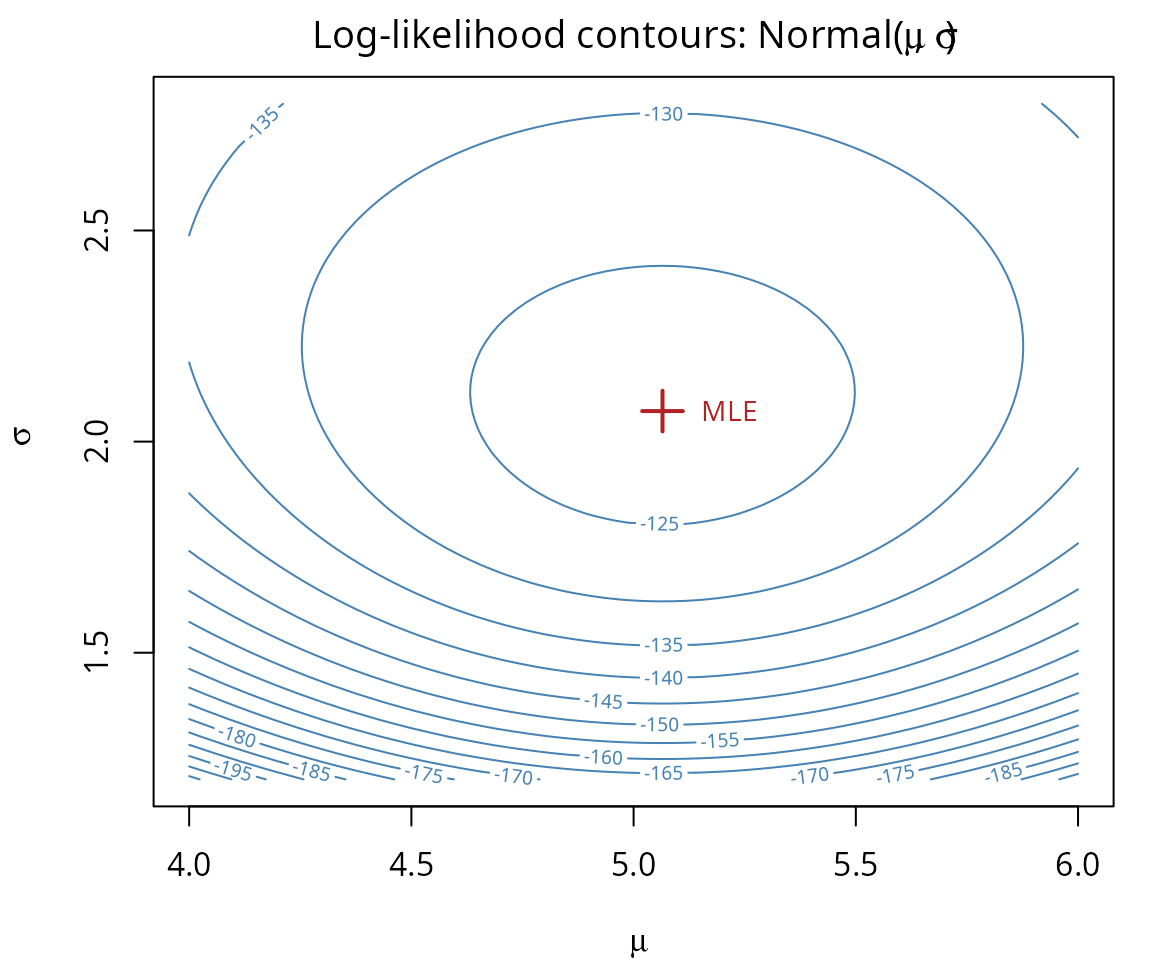

Newton-Raphson convergence path

We can visualize how Newton-Raphson converges to the MLE by recording the parameter estimates at each iteration and overlaying them on the contour plot:

# Newton-Raphson with trace
newton_raphson_trace <- function(f, theta0, tol = 1e-8, max_iter = 50) {
  theta <- theta0
  trace <- list(theta)
  for (iter in seq_len(max_iter)) {
    g <- gradient(f, theta)
    H <- hessian(f, theta)
    step <- solve(H, g)
    theta <- theta - step
    trace[[iter + 1L]] <- theta
    if (max(abs(g)) < tol) break
  }
  list(estimate = theta, iterations = iter, trace = do.call(rbind, trace))
}

result_trace <- newton_raphson_trace(ll_normal_2, c(3, 1))

par(mar = c(4, 4, 2, 1))
contour(mu_grid, sigma_grid, ll_surface, nlevels = 25,
        xlab = expression(mu), ylab = expression(sigma),
        main = "Newton-Raphson convergence path",
        col = "grey70")
lines(result_trace$trace[, 1], result_trace$trace[, 2],
      col = "firebrick", lwd = 2, type = "o", pch = 19, cex = 0.8)
points(result_trace$trace[1, 1], result_trace$trace[1, 2],
       pch = 17, col = "orange", cex = 1.5)
points(mle_mu, mle_sigma, pch = 3, col = "steelblue", cex = 2, lwd = 2)
legend("topright",
       legend = c("N-R path", "Start", "MLE"),
       col = c("firebrick", "orange", "steelblue"),
       pch = c(19, 17, 3), lty = c(1, NA, NA), lwd = c(2, NA, 2),
       bty = "n")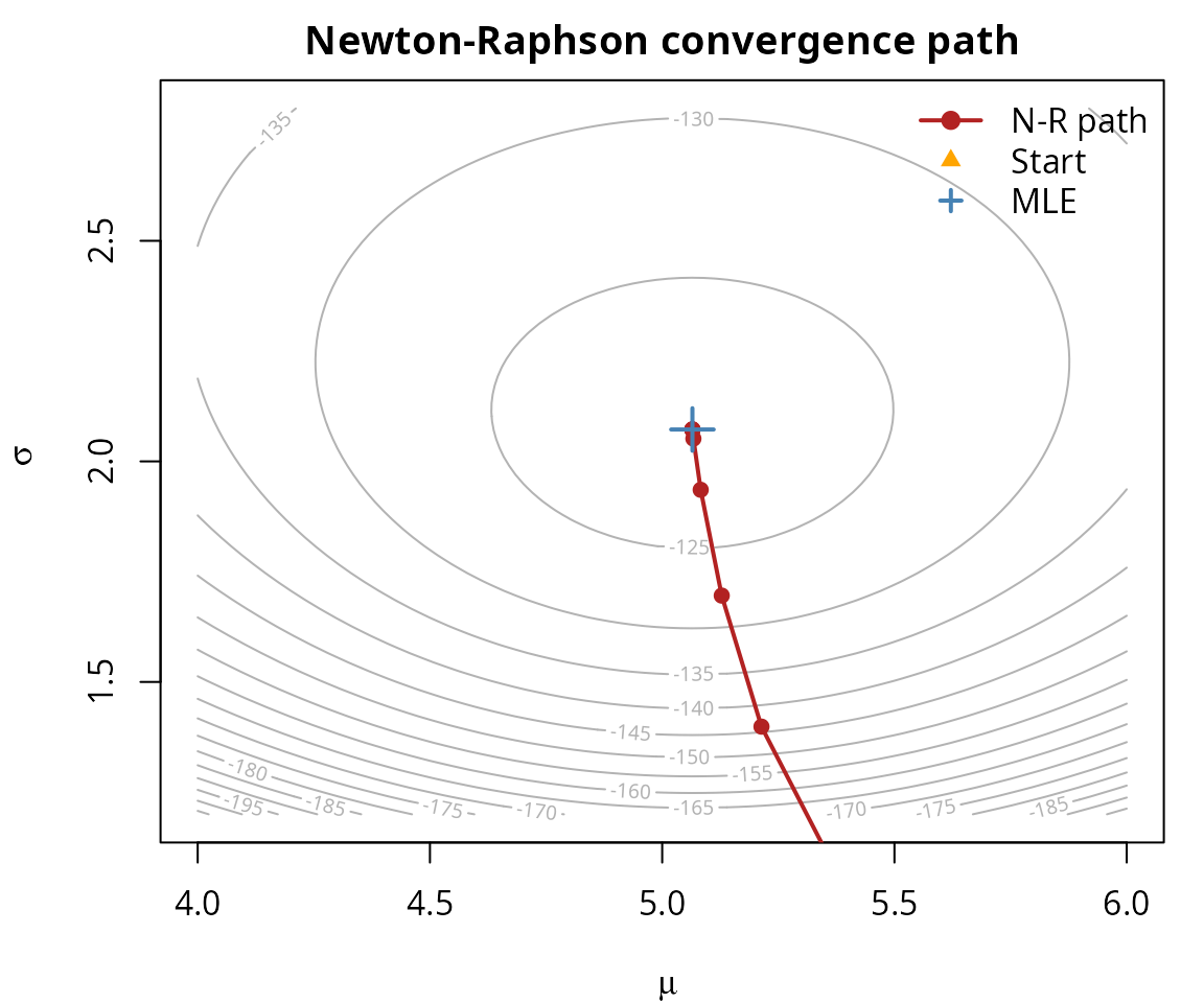

Newton-Raphson converges in 10 iterations — fast quadratic convergence is a hallmark of having exact gradient and Hessian information from AD.

`jacobian()`: differentiating a vector-valued function

When a function returns a vector (or list) of outputs, jacobian() computes the full Jacobian matrix $J_{ij} = \partial f_i / \partial x_j$ :

# f: R^2 -> R^3
f_vec <- function(x) {
  a <- x[1]; b <- x[2]
  list(a * b, a^2, sin(b))
}

J <- jacobian(f_vec, c(2, pi/4))
J
#>           [,1]      [,2]
#> [1,] 0.7853982 2.0000000
#> [2,] 4.0000000 0.0000000
#> [3,] 0.0000000 0.7071068

# Analytical Jacobian at (2, pi/4):
# Row 1: d(a*b)/da = b = pi/4,  d(a*b)/db = a = 2
# Row 2: d(a^2)/da = 2a = 4,    d(a^2)/db = 0
# Row 3: d(sin(b))/da = 0,      d(sin(b))/db = cos(b)

This is useful for sensitivity analysis, implicit differentiation, or any application where a function maps multiple inputs to multiple outputs.

Summary

Across five models of increasing complexity, several patterns emerge:

AD matches analytical derivatives to machine precision. Whether the function involves simple polynomials (Normal), special functions (lgamma in Gamma), or loops over observations (logistic regression), gradient() and hessian() return exact results.
Finite differences introduce step-size-dependent error. For simple models the error is negligible ( $\sim 10^{-10}$ ), but for loop-based functions it grows to $\sim 10^{-5}$ — large enough to affect optimization convergence and standard error estimates.
jacobian() extends to vector-valued functions. For functions $f: \mathbb{R}^n \to \mathbb{R}^m$ , jacobian() computes the full $m \times n$ Jacobian matrix using $n$ forward passes.
Newton-Raphson with AD gradients converges in few iterations. The exact Hessian provides the quadratic convergence that Newton’s method promises in theory — no line search or quasi-Newton approximation needed.