Plot Optimization Convergence

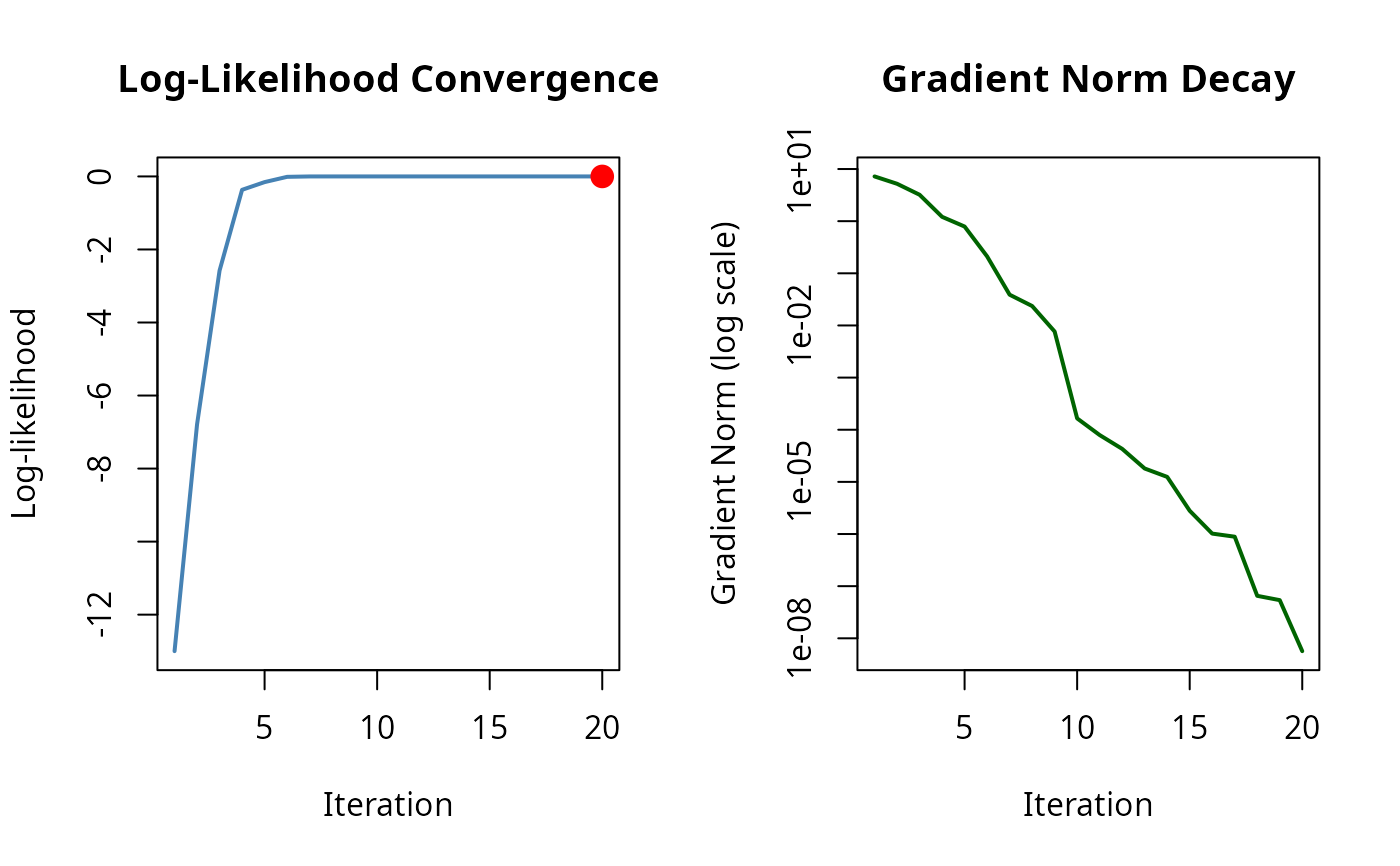
Visualizes the optimization trajectory from an MLE result with tracing enabled. Shows log-likelihood progression, gradient norm decay, and optionally the parameter path (for 2D problems).

Usage

# S3 method for class 'mle_numerical'
plot(x, which = c("loglike", "gradient"), main = NULL, ...)

Arguments

x

An mle_numerical result object with trace_data

which

Character vector specifying which plots to show: "loglike" (log-likelihood), "gradient" (gradient norm), "path" (2D parameter path)

main

Optional title

...

Additional arguments passed to plot

Value

Invisibly returns the trace data

Details

This function requires that the solver was run with tracing enabled via mle_trace(). Without trace data, the function will warn and return invisibly.

The "path" plot is only shown for 2D parameter problems.

Examples

# \donttest{
# Enable tracing when solving
problem <- mle_problem(
  loglike = function(theta) -sum((theta - c(3, 2))^2),
  constraint = mle_constraint(support = function(theta) TRUE)
)
trace_cfg <- mle_trace(values = TRUE, gradients = TRUE, path = TRUE)
result <- gradient_ascent(max_iter = 50)(problem, c(0, 0), trace = trace_cfg)

# Plot convergence diagnostics
plot(result)

# }