When to Use This Package
Use compositional.mle when:
- Multi-modal likelihoods: Your likelihood surface has multiple local optima and you need global search strategies (simulated annealing, random restarts)
- Coarse-to-fine optimization: You want to start with a rough global search and progressively refine with local methods
- Comparing strategies: You’re unsure which optimizer works best and want to race them automatically
- Building robust pipelines: You need reliable estimation that handles edge cases gracefully
- Research/experimentation: You want to explore optimization strategies and visualize convergence
Stick with optim() when:
- You have a simple, well-behaved likelihood with a single optimum
- You know exactly which method works and don’t need composition
Example: Why Composition Matters
library(compositional.mle)

# A tricky bimodal likelihood
set.seed(42)
bimodal_loglike <- function(theta) {
  # Two peaks: one at theta=2, one at theta=8
  log(0.3 * dnorm(theta, 2, 0.5) + 0.7 * dnorm(theta, 8, 0.5))
}

problem <- mle_problem(
 loglike = bimodal_loglike,
  constraint = mle_constraint(support = function(theta) TRUE)
)

# Single gradient ascent gets trapped at local optimum
result_local <- gradient_ascent()(problem, theta0 = 0)

# Simulated annealing + gradient ascent finds global optimum
strategy <- sim_anneal(temp_init = 5, max_iter = 200) %>>% gradient_ascent()
result_global <- strategy(problem, theta0 = 0)

cat("Local search found:", round(result_local$theta.hat, 2),
    "(log-lik:", round(result_local$loglike, 2), ")\n")
#> Local search found: 2 (log-lik: -1.43 )
cat("Global strategy found:", round(result_global$theta.hat, 2),
    "(log-lik:", round(result_global$loglike, 2), ")\n")
#> Global strategy found: 2 (log-lik: -1.43 )
Installation
# From CRAN (when available)
install.packages("compositional.mle")

# Development version
devtools::install_github("queelius/compositional.mle")
Design Philosophy
Following SICP principles, the package provides: 1. Primitive solvers - gradient_ascent(), newton_raphson(), bfgs(), sim_anneal(), etc. 2. Composition operators - %>>% (sequential), %|% (race), with_restarts() 3. Closure property - Combining solvers yields a solver
Quick Start
# Generate sample data
set.seed(42)
x <- rnorm(100, mean = 5, sd = 2)

# Define the problem (separate from solver strategy)
problem <- mle_problem(
  loglike = function(theta) {
    if (theta[2] <= 0) return(-Inf)
    sum(dnorm(x, theta[1], theta[2], log = TRUE))
  },
  score = function(theta) {
    mu <- theta[1]; sigma <- theta[2]; n <- length(x)
    c(sum(x - mu) / sigma^2,
      -n / sigma + sum((x - mu)^2) / sigma^3)
  },
  constraint = mle_constraint(
    support = function(theta) theta[2] > 0,
    project = function(theta) c(theta[1], max(theta[2], 1e-8))
  )
)

# Simple solve
result <- gradient_ascent()(problem, theta0 = c(0, 1))
result$theta.hat
#> [1] 5.065030 2.072274
Composing Solvers
Sequential Chaining (%>>%)
Chain solvers for coarse-to-fine optimization:
# Grid search -> gradient ascent -> Newton-Raphson
strategy <- grid_search(lower = c(-10, 0.5), upper = c(10, 5), n = 5) %>>%
  gradient_ascent(max_iter = 50) %>>%
  newton_raphson(max_iter = 20)

result <- strategy(problem, theta0 = c(0, 1))
result$theta.hat
#>     Var1     Var2
#> 5.065030 2.072274
Parallel Racing (%|%)
Race multiple methods, keep the best:
# Try multiple approaches, pick winner by log-likelihood
strategy <- gradient_ascent() %|% bfgs() %|% nelder_mead()

result <- strategy(problem, theta0 = c(0, 1))
c(result$theta.hat, loglike = result$loglike)
#>                             loglike
#>    5.065030    2.072274 -214.758518
Random Restarts
Escape local optima with multiple starting points:
strategy <- with_restarts(
  gradient_ascent(),
  n = 10,
  sampler = uniform_sampler(c(-10, 0.5), c(10, 5))
)

result <- strategy(problem, theta0 = c(0, 1))
result$theta.hat
#> [1] 5.065030 2.072274
Visualization
Track and visualize the optimization path:
# Enable tracing
trace_cfg <- mle_trace(values = TRUE, gradients = TRUE, path = TRUE)
result <- gradient_ascent(max_iter = 50)(problem, c(0, 1), trace = trace_cfg)

# Plot convergence
plot(result, which = c("loglike", "gradient"))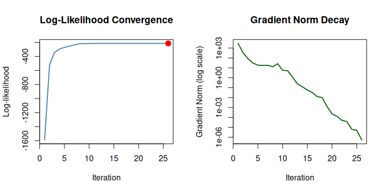
Extract trace as data frame for custom analysis:
path_df <- optimization_path(result)
head(path_df)
#>   iteration    loglike  grad_norm   theta_1  theta_2
#> 1         1 -1589.3361 2938.86063 0.0000000 1.000000
#> 2         2  -518.7066  334.47435 0.1723467 1.985036
#> 3         3  -344.5384   84.57555 0.5435804 2.913576
#> 4         4  -293.8366   30.83372 1.1733478 3.690360
#> 5         5  -271.7336   18.65296 2.1001220 4.065978
#> 6         6  -254.0618   17.83778 3.0615865 3.791049
Available Solvers
| Factory | Method | Best For |
|---|---|---|
gradient_ascent() |
Steepest ascent with line search | General purpose, smooth likelihoods |
newton_raphson() |
Second-order Newton | Fast convergence near optimum |
bfgs() |
Quasi-Newton BFGS | Good balance of speed/robustness |
lbfgsb() |
L-BFGS-B with box constraints | High-dimensional, bounded parameters |
nelder_mead() |
Simplex (derivative-free) | Non-smooth or noisy likelihoods |
sim_anneal() |
Simulated annealing | Global optimization, multi-modal |
coordinate_ascent() |
One parameter at a time | Different parameter scales |
grid_search() |
Exhaustive grid | Finding starting points |
random_search() |
Random sampling | High-dimensional exploration |
Function Transformers
# Stochastic gradient (mini-batching for large data)
loglike_sgd <- with_subsampling(loglike, data = x, subsample_size = 32)

# Regularization
loglike_l2 <- with_penalty(loglike, penalty_l2(), lambda = 0.1)
loglike_l1 <- with_penalty(loglike, penalty_l1(), lambda = 0.1)
Documentation
- Full documentation: https://queelius.github.io/compositional.mle/
- Vignettes: