Designing Optimization Strategies

Introduction

This vignette shows how to design effective optimization strategies by composing solvers. We’ll cover:

Diagnosing convergence problems
Building robust pipelines
Benchmarking solver combinations
Handling common failure modes

The Problem: Why Composition?

Consider fitting a mixture of normals - a notoriously multi-modal problem:

# Generate mixture data
x_mix <- c(rnorm(70, mean = 0, sd = 1), rnorm(30, mean = 5, sd = 1.5))

# Log-likelihood for 2-component Gaussian mixture
mixture_loglike <- function(theta) {
  mu1 <- theta[1]; s1 <- theta[2]
  mu2 <- theta[3]; s2 <- theta[4]
  pi1 <- theta[5]

  if (s1 <= 0 || s2 <= 0 || pi1 <= 0 || pi1 >= 1) return(-Inf)

  # Log-sum-exp for numerical stability
  log_p1 <- log(pi1) + dnorm(x_mix, mu1, s1, log = TRUE)
  log_p2 <- log(1 - pi1) + dnorm(x_mix, mu2, s2, log = TRUE)
  log_max <- pmax(log_p1, log_p2)
  sum(log_max + log(exp(log_p1 - log_max) + exp(log_p2 - log_max)))
}

problem_mix <- mle_problem(
  loglike = mixture_loglike,
  constraint = mle_constraint(
    support = function(theta) theta[2] > 0 && theta[4] > 0 &&
                              theta[5] > 0 && theta[5] < 1,
    project = function(theta) c(theta[1], max(theta[2], 0.1), theta[3],
                                max(theta[4], 0.1), min(max(theta[5], 0.01), 0.99))
  )
)

Single Solver: Often Fails

# Random starting point
theta0 <- c(-2, 1, 3, 1, 0.5)

result_simple <- gradient_ascent(max_iter = 100)(problem_mix, theta0)

cat("Simple gradient ascent:\n")
#> Simple gradient ascent:
cat("  mu1 =", round(result_simple$theta.hat[1], 2),
    " mu2 =", round(result_simple$theta.hat[3], 2), "\n")
#>   mu1 = 0.12  mu2 = 2.66
cat("  Log-likelihood:", round(result_simple$loglike, 2), "\n")
#>   Log-likelihood: -219.25

The result depends heavily on the starting point, and we often get stuck at local optima.

Strategy 1: Coarse-to-Fine

Start with a rough global search, then refine:

# K-means for smart initialization
km <- kmeans(x_mix, centers = 2)
mu1_init <- min(km$centers)
mu2_init <- max(km$centers)
s1_init <- sd(x_mix[km$cluster == which.min(km$centers)])
s2_init <- sd(x_mix[km$cluster == which.max(km$centers)])
pi_init <- mean(km$cluster == which.min(km$centers))

theta_init <- c(mu1_init, s1_init, mu2_init, s2_init, pi_init)

# Coarse-to-fine: random search -> gradient ascent
strategy <- random_search(
  sampler = function() c(runif(1, -5, 10), runif(1, 0.5, 3),
                         runif(1, -5, 10), runif(1, 0.5, 3),
                         runif(1, 0.2, 0.8)),
  n = 50
) %>>% gradient_ascent(max_iter = 200)

result_coarse <- strategy(problem_mix, theta_init)

cat("Coarse-to-fine strategy:\n")
#> Coarse-to-fine strategy:
cat("  mu1 =", round(result_coarse$theta.hat[1], 2),
    " mu2 =", round(result_coarse$theta.hat[3], 2), "\n")
#>   mu1 = 0.08  mu2 = 4.96
cat("  Log-likelihood:", round(result_coarse$loglike, 2), "\n")
#>   Log-likelihood: -215.73

Strategy 2: Multiple Restarts

Run gradient ascent from many starting points:

# Custom sampler for mixture parameters
mixture_sampler <- function() {
  c(runif(1, -5, 10),    # mu1
    runif(1, 0.5, 3),     # sigma1
    runif(1, -5, 10),     # mu2
    runif(1, 0.5, 3),     # sigma2
    runif(1, 0.2, 0.8))   # pi
}

strategy <- with_restarts(
  gradient_ascent(max_iter = 100),
  n = 20,
  sampler = mixture_sampler
)

result_restarts <- strategy(problem_mix, theta_init)

cat("Random restarts (20 starts):\n")
#> Random restarts (20 starts):
cat("  mu1 =", round(result_restarts$theta.hat[1], 2),
    " mu2 =", round(result_restarts$theta.hat[3], 2), "\n")
#>   mu1 = 0.08  mu2 = 4.96
cat("  Log-likelihood:", round(result_restarts$loglike, 2), "\n")
#>   Log-likelihood: -215.73
cat("  Best restart:", result_restarts$best_restart, "of", result_restarts$n_restarts, "\n")
#>   Best restart: 1 of 20

Strategy 3: Racing Solvers

When unsure which method works best, race them:

strategy <- gradient_ascent() %|% bfgs() %|% nelder_mead()

result_race <- strategy(problem_mix, theta_init)

cat("Racing strategy:\n")
#> Racing strategy:
cat("  Winner:", result_race$solver, "\n")
#>   Winner: gradient_ascent
cat("  mu1 =", round(result_race$theta.hat[1], 2),
    " mu2 =", round(result_race$theta.hat[3], 2), "\n")
#>   mu1 = 0.08  mu2 = 4.96
cat("  Log-likelihood:", round(result_race$loglike, 2), "\n")
#>   Log-likelihood: -215.73

Strategy 4: Global + Local

Combine simulated annealing for global exploration with gradient ascent for local refinement:

strategy <- sim_anneal(temp_init = 10, cooling_rate = 0.95, max_iter = 500) %>>%
  gradient_ascent(max_iter = 100)

result_global <- strategy(problem_mix, theta_init)

cat("Global + local strategy:\n")
#> Global + local strategy:
cat("  mu1 =", round(result_global$theta.hat[1], 2),
    " mu2 =", round(result_global$theta.hat[3], 2), "\n")
#>   mu1 = 0.08  mu2 = 4.96
cat("  Log-likelihood:", round(result_global$loglike, 2), "\n")
#>   Log-likelihood: -215.73

Diagnosing Convergence

Use tracing to understand optimization behavior:

# Enable full tracing
trace_cfg <- mle_trace(values = TRUE, gradients = TRUE, path = TRUE)

# Simple problem for clear visualization
simple_problem <- mle_problem(
  loglike = function(theta) -sum((theta - c(3, 2))^2),
  score = function(theta) -2 * (theta - c(3, 2)),
  constraint = mle_constraint(support = function(theta) TRUE)
)

result_traced <- gradient_ascent(max_iter = 30)(
  simple_problem, c(-2, -1), trace = trace_cfg
)

# Visualize convergence
plot(result_traced, which = c("loglike", "path"))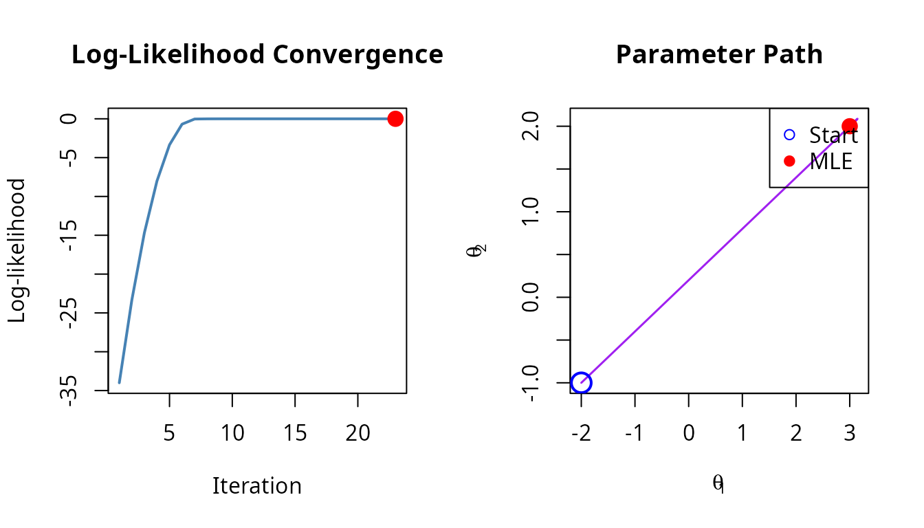

Extracting Trace Data

path_df <- optimization_path(result_traced)
head(path_df)
#>   iteration     loglike grad_norm    theta_1     theta_2
#> 1         1 -34.0000000 11.661904 -2.0000000 -1.00000000
#> 2         2 -23.3380962  9.661904 -1.1425071 -0.48550424
#> 3         3 -14.6761924  7.661904 -0.2850141  0.02899151
#> 4         4  -8.0142886  5.661904  0.5724788  0.54348727
#> 5         5  -3.3523848  3.661904  1.4299717  1.05798302
#> 6         6  -0.6904811  1.661904  2.2874646  1.57247878

# Check convergence rate
if (nrow(path_df) > 5) {
  improvement <- diff(path_df$loglike)
  cat("\nLog-likelihood improvement per iteration:\n")
  print(round(improvement[1:min(5, length(improvement))], 4))
}
#> 
#> Log-likelihood improvement per iteration:
#> [1] 10.6619  8.6619  6.6619  4.6619  2.6619

Benchmarking Strategies

Compare different strategies on the same problem:

# Test problem: bimodal likelihood
bimodal <- mle_problem(
  loglike = function(theta) {
    log(0.3 * dnorm(theta, 2, 0.5) + 0.7 * dnorm(theta, 7, 0.5))
  },
  constraint = mle_constraint(support = function(theta) TRUE)
)

# Strategies to compare
strategies <- list(
  "Gradient Ascent" = gradient_ascent(max_iter = 100),
  "BFGS" = bfgs(),
  "Nelder-Mead" = nelder_mead(),
  "SA + GA" = sim_anneal(max_iter = 200) %>>% gradient_ascent(),
  "Restarts (5)" = with_restarts(gradient_ascent(), n = 5,
                                  sampler = function() runif(1, -5, 15))
)

# Run each strategy multiple times
results <- data.frame(
  Strategy = character(),
  LogLike = numeric(),
  Theta = numeric(),
  stringsAsFactors = FALSE
)

for (name in names(strategies)) {
  for (rep in 1:3) {
    set.seed(rep * 100)
    theta0 <- runif(1, -5, 15)
    result <- tryCatch(
      strategies[[name]](bimodal, theta0),
      error = function(e) NULL
    )
    if (!is.null(result)) {
      results <- rbind(results, data.frame(
        Strategy = name,
        LogLike = result$loglike,
        Theta = result$theta.hat[1],
        stringsAsFactors = FALSE
      ))
    }
  }
}
#> Warning in optim(par = theta0, fn = fn, method = "Nelder-Mead", control = list(maxit = max_iter, : one-dimensional optimization by Nelder-Mead is unreliable:
#> use "Brent" or optimize() directly
#> Warning in optim(par = theta0, fn = fn, method = "Nelder-Mead", control = list(maxit = max_iter, : one-dimensional optimization by Nelder-Mead is unreliable:
#> use "Brent" or optimize() directly
#> Warning in optim(par = theta0, fn = fn, method = "Nelder-Mead", control = list(maxit = max_iter, : one-dimensional optimization by Nelder-Mead is unreliable:
#> use "Brent" or optimize() directly

# Summarize results
library(dplyr)
#> 
#> Attaching package: 'dplyr'
#> The following objects are masked from 'package:stats':
#> 
#>     filter, lag
#> The following objects are masked from 'package:base':
#> 
#>     intersect, setdiff, setequal, union
results %>%
  group_by(Strategy) %>%
  summarize(
    MeanLogLike = round(mean(LogLike), 2),
    BestTheta = round(Theta[which.max(LogLike)], 2),
    .groups = "drop"
  ) %>%
  arrange(desc(MeanLogLike))
#> # A tibble: 5 × 3
#>   Strategy        MeanLogLike BestTheta
#>   <chr>                 <dbl>     <dbl>
#> 1 Restarts (5)          -0.58         7
#> 2 BFGS                  -0.86         7
#> 3 Gradient Ascent       -0.86         7
#> 4 Nelder-Mead           -0.86         7
#> 5 SA + GA               -0.86         7

Best Practices

1. Start Simple, Add Complexity

# First try: simple gradient ascent
result <- gradient_ascent()(problem, theta0)

# If it fails, add restarts
result <- with_restarts(gradient_ascent(), n = 10, sampler = my_sampler)(problem, theta0)

# If still failing, try global + local
result <- (sim_anneal() %>>% gradient_ascent())(problem, theta0)

2. Use Domain Knowledge for Initialization

# Method of moments for mixture initialization
m <- mean(data); v <- var(data)
theta0 <- c(m - sqrt(v), sqrt(v), m + sqrt(v), sqrt(v), 0.5)

3. Match Solver to Problem

Problem Type	Recommended Strategy
Smooth, unimodal	`gradient_ascent()` or `bfgs()`
Multi-modal	`with_restarts()` or `sim_anneal() %>>% gradient_ascent()`
High-dimensional	`lbfgsb()` or `coordinate_ascent()`
Non-smooth	`nelder_mead()`
Unknown	`gradient_ascent() %\|% bfgs() %\|% nelder_mead()`

4. Monitor Convergence

Always enable tracing during development:

result <- solver(problem, theta0, trace = mle_trace(values = TRUE, gradients = TRUE))
plot(result)

Summary

The compositional approach lets you:

Combine strengths: Global search + local refinement
Handle uncertainty: Race multiple methods
Build robustness: Multiple restarts
Diagnose issues: Full tracing and visualization

Start with simple strategies and add complexity only when needed.

Alexander Towell

2026-01-31