Introduction
To demonstrate the R package algebraic.mle, we consider the relatively simple case of a random sample from i.i.d. normally distributed random variables. First, we load the R package algebraic.mle with:
library(algebraic.mle)
library(boot)
Generating a sample
We define the parameters of the i.i.d. random sample with:
n <- 50
theta <- c(4,2)
We generate a random sample \(X_i \sim \operatorname{N}(\mu=4,\sigma^2=2)\) for \(i=1,\ldots,n\) with:
We have observed a sample of size \(n=50\). We show some observations from this sample (data frame) with:
head(x,n=4)
#> [1] 6.02 1.30 3.47 2.94
We show a histogram of the sample with:
hist(x)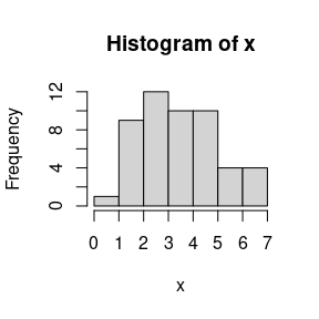
We see the characteristic bell shaped curve of the normal distribution. If we did not a prior know that the data was normally distributed, this would be evidence that the normal distribution is a good fit to the data.
Maximum likelihood estimation
If we would like to estimate \(\theta=(4, 2)'\), we can do so using maximum likelihood estimation as implemented by the algebraic.mle package:
theta.hat <- mle_normal(x)
summary(theta.hat)
#> Maximum likelihood estimator of type mle_normal is normally distributed.
#> The estimates of the parameters are given by:
#>   mu  var
#> 3.68 1.63
#> The standard error is  0.18 0.326 .
#> The asymptotic 95% confidence interval of the parameters are given by:
#>      2.5% 97.5%
#> mu  3.321  4.05
#> var 0.974  2.28
#> The MSE of the individual componetns in a multivariate estimator is:
#> [1] 0.0326 0.1071
#> The MSE of the estimator is  0.0326 -0.0000000000000000185 0.00000000000000000568 0.107 .
#> The log-likelihood is  -83.1 .
#> The AIC is  170 .
We can show the point estimate given data x with:
point(theta.hat)
#>   mu  var
#> 3.68 1.63
We can show the Fisher information matrix (FIM) and variance-covariance matrix with:
fim(theta.hat)
#>                      [,1]                [,2]
#> [1,] 30.70482653349504432 0.00000000000000536
#> [2,]  0.00000000000000536 9.42786372452020238
vcov(theta.hat)
#>                        [,1]                   [,2]
#> [1,]  0.0325681696624837702 0.00000000000000000568
#> [2,] -0.0000000000000000185 0.10606856751643294057
We can show the confidence intervals with:
confint(theta.hat)
#>      2.5% 97.5%
#> mu  3.321  4.05
#> var 0.974  2.28
A nice property of MLEs is that, asymptotically, they converge to a normal distribution with a mean given by the true parameter, in this case \(\theta = (\mu,\sigma^2)'\), and a variance-covariance given by the inverse of the Fisher information matrix evaluated at \(\theta\). This is how we estimated the confidence intervals and other statistics above.
Performance measures of the MLE
We do not know \(\theta\), but we may estimate it from a sample, and thus we may approximate the sampling distribution of \(\hat\theta\) with \(\mathcal{N}(\hat\theta,I^{-1}(\hat\theta))\).
Let \(F\) denote the true distribution function such that \(X_j \sim F\) for all \(j\). Suppose we have some population parameter \(\theta = t(F)\) and an estimator of \(\theta\) given by \(\hat\theta = s(\{X_1,\ldots,X_n\})\). A reasonable requirement for an estimator \(\hat\theta\) is that it converges to the true parameter value \(\theta\) as we collect more and more data. In particular, we say that it is a consistent estimator of \(\theta\) if \(\hat\theta\) converges in probability to \(\theta\), denoted by \(\hat\theta \overset{p}{\mapsto} \theta\).
If the regularity conditions hold for the MLE, then \(\hat\theta\) is a consistent estimator of \(\theta\). However, for finite sample sizes, the estimator may be biased. The bias of \(\hat\theta\) with respect to \(\theta\) is defined as \[ \operatorname{bias}(\hat\theta,\theta) = E(\hat\theta) - \theta, \] where \(\operatorname{bias}(\hat\theta,\theta) = 0\) indicates that \(\hat\theta\) is an unbiased estimator of \(\theta\).
As a function of the true distribution \(F\), the bias is unknown and is not a statistic. However, in the case of the normal, \(\hat\mu\) is unbiased and, analytically, the bias of \(\hat\sigma^2\) is given by \(-\frac{1}{n} \sigma^2\):
bias(theta.hat,theta)
#> [1]  0.00 -0.04
If \(\sigma^2\) is not known, we may estimate it by using replacing \(\hat\sigma^2\) instead:
bias(theta.hat)
#>             var
#>  0.0000 -0.0326
The mean squared error (MSE) is another performance measure of an estimator. It is given by \[ \operatorname{mse}(\hat\theta) = E\bigl\{(\hat\theta - \theta)^T(\hat\theta - \theta)\bigr\}, \] Another way to compute the MSE is given by \[ \operatorname{mse}(\hat\theta) = \operatorname{trace}(\operatorname{cov}(\hat\theta) + \operatorname{bias}(\hat\theta)^T \operatorname{bias}(\hat\theta). \]
Here’s R code to compute the MSE of \(\hat\theta\):
mse(theta.hat)         # estimate of MSE
#>                                                var
#> [1,]  0.0325681696624837702 0.00000000000000000568
#> [2,] -0.0000000000000000185 0.10712925319159727344
mse(theta.hat, theta)  # true MSE
#>                        [,1]                   [,2]
#> [1,]  0.0325681696624837702 0.00000000000000000568
#> [2,] -0.0000000000000000185 0.10766856751643294476
This looks to be a pretty good estimate of the true MSE.
Invariance property of the MLE
An interesting property of an MLE \(\hat\theta\) is that the MLE of \(f(\theta)\) is given by \(f(\hat\theta)\). What is the distribution of \(f(\hat\theta)\)? Asymptotically, it is normally distributed with a mean given by \(f(\theta)\) and a variace-covariance given by the covariance of the sampling distribution of \(f(\hat\theta)\). We provide two methods to compute the variance-covariance.
Delta method
If \(f\) is differentiable, the variance-covariance is given by \[ \operatorname{var}(f(\hat\theta)) = \operatorname{E}\bigl\{ \bigl(f(\hat\theta) - f(\theta)\bigr)^2\bigr\} = \operatorname{E}\bigl\{J_f(\hat\theta) I(\hat\theta)^{-1} J_f(\hat\theta)^T\bigr\}. \] Here, \(J_f(\hat\theta)\) is the Jacobian of \(f\) evaluated at \(\hat\theta\).
Monte-carlo method
The delta method requires that \(f\) be differentiable, but we may use the Monte-carlo method to estimate the distribution of \(f(\hat\theta)\) for any function \(f\). We simply sample from the MLE of \(\hat\theta\) and apply \(f\) to its point estimates and take the covariance of the sample.
Next, we show how to compute the sampling distribution of \(g(\hat\theta)\) for some function \(g\) and some MLE \(\hat\theta\) using both the delta and mc methods.
Example 1
Let \(g(\theta) = A \theta + b\) for some matrix \(A\) and vector \(b\). (This is a simple linear transformation of \(\theta\).) We can define \(g\) in R with:
We compute the MLE of \(g(\theta)\) with:
g.mc <- rmap(theta.hat,g,n=100000L)
g.delta <- rmap(theta.hat,g,method="delta")

round(vcov(g.mc),digits=3)
#>       [,1]  [,2]  [,3]  [,4]
#> [1,] 0.131 0.196 0.001 0.001
#> [2,] 0.196 0.295 0.001 0.002
#> [3,] 0.001 0.001 0.426 0.640
#> [4,] 0.001 0.002 0.640 0.960
round(vcov(g.delta),digits=3)
#>       [,1]  [,2]  [,3]  [,4]
#> [1,] 0.130 0.195 0.000 0.000
#> [2,] 0.195 0.293 0.000 0.000
#> [3,] 0.000 0.000 0.424 0.636
#> [4,] 0.000 0.000 0.636 0.955
They are pretty close.
Weighted MLE: a weighted sum of maximum likelihood estimators
Since the variance-covariance of an MLE is inversely proportional to the Fisher information that the MLE is defined with respect to, we can combine multiple MLEs of \(\theta\), each of which may be defined with respect to a different kind of sample, to arrive at the MLE that incorporates the Fisher information in all of those samples.
Consider \(k\) mutually independent MLEs of parameter \(\theta\), \(\hat\theta_1,\ldots,\hat\theta_k\), where \(\hat\theta_j \sim N(\theta,I_j^{-1}(\theta))\). Then, the sampling MLE of \(\theta\) that incorporates all of the data in \(\hat\theta_1,\ldots,\hat\theta_k\) is given by the inverse-variance weighted mean, \[ \hat\theta_w = \left(\sum_{j=1}^k I_j(\theta)\right)^{-1} \left(\sum_{j=1}^k I_j(\theta) \hat\theta_j\right), \] which, asymptotically, has an expected value of \(\theta\) and a variance-covariance of \(\left(\sum_{j=1}^k I_j(\theta)\right)^{-1}\).
Example 2
To evaluate the performance of the weighted MLE, we generate a sample of \(N=1000\) observations from \(\mathcal{N}(\theta)\) and compute the MLE for the observed sample, denoted by \(\hat\theta\).
We then divide the observed sample into \(r=5\) sub-samples, each of size \(N/r=100\), and compute the MLE for each sub-sampled, denoted by \(\theta^{(1)},\ldots,\theta^{(r)}\).
Finally, we do a weighted combination these MLEs to form the weighted MLE, denoted by \(\theta_w\):
N <- 100
r <- 5
samp <- rnorm(N, mean = theta[1], sd = sqrt(theta[2]))
samp.sub <- matrix(samp, nrow = r)
mles.sub <- list(length = r)
for (i in 1:r)
    mles.sub[[i]] <- mle_normal(samp.sub[i,])

mle.wt <- mle_weighted(mles.sub)
mle <- mle_normal(samp)
We show the results in the following R code. First, we show the weighted MLE and its MSE:
#point(mle.wt)
#mse(mle.wt)
The MLE for the total sample and its MSE is:
point(mle)
#>   mu  var
#> 4.25 1.93
mse(mle)
#>                                               var
#> [1,]  0.019294470272057680 0.00000000000000000284
#> [2,] -0.000000000000000011 0.07482759319894285999
We see that \(\hat\theta\) and \(\hat\theta_w\) model approximately the same sampling distribution when estimating \(\theta\) given i.i.d. samples.
Bootstrapping the MLEs
Let’s compare the earlier results that relied on the large sampling assumption with the bootstrapped MLE using mle_boot. First, mle_boot is just a wrapper for boot objects or objects like boot. Thus to use mle_boot, we first need to call boot to bootstrap our MLE for the normal.
one with mle_normal: we just need to wrap it in a function that takes the data as input and returns the MLE of the parameters and then pass it to mle_boot constructor:
theta.boot <- mle_boot(
    boot(data = x,
         statistic = function(x, i) point(mle_normal(x[i])),
         R = 1000))
We already printed out the theta.boot object, which provided a lot of information about it, but we can obtain specified statistics from the Bootstrap MLE using the standard interface in algorithmic.mle, e.g.:
confint(theta.boot) # confidence interval
#> BOOTSTRAP CONFIDENCE INTERVAL CALCULATIONS
#> Based on 1000 bootstrap replicates
#>
#> CALL :
#> boot.ci(boot.out = x, conf = level)
#>
#> Intervals :
#> Level      Normal              Basic             Studentized
#> 95%   ( 3.34,  4.03 )   ( 3.34,  4.02 )   ( 3.36,  4.05 )
#>
#> Level     Percentile            BCa
#> 95%   ( 3.35,  4.02 )   ( 3.36,  4.03 )
#> Calculations and Intervals on Original Scale
(point(theta.boot)) # point estimate
#>   mu  var
#> 3.68 1.63
(vcov(theta.boot)) # variance-covariance matrix
#>        [,1]   [,2]
#> [1,] 0.0303 0.0192
#> [2,] 0.0192 0.1157
(se(theta.boot)) # standard error
#> [1] 0.174 0.340
(bias(theta.boot)) # bias
#>       mu      var
#> -0.00182 -0.04896
(mse(theta.boot)) # mean squared error
#> [1] 0.148
We see that, for the most part, the results are similar to those obtained using the large sampling assumption.
Prediction intervals
Frequently, we are actually interested in predicting the outcome of the random variable (or vector) that we are estimating the parameters of.
We observed a sample \(\mathcal{D} = \{T_i\}_{i=1}^n\) where \(T_i \sim N(\mu,\sigma^2)\), \(\theta = (\mu,\sigma^2)^T\) is not known. We compute the MLE of \(\theta\), which, asymptotically, is normally distributed with a mean \(\theta\) and a variance-covariance \(I^{-1}(\theta)/n\).
We wish to model the uncertainty of a new observation, \(\hat{T}_{n+1}|\mathcal{D}\). We do so by considering both the uncertainty inherent to the Normal distribution and the uncertainty of our estimate \(\hat\theta\) of \(\theta\). In particular, we let \(\hat{T}_{n+1}|\hat\theta \sim N(\hat\mu,\hat\sigma^2)\) and \(\hat\theta \sim N(\theta,I^{-1}(\theta)/n)\) (the sampling distribution of the MLE). Then, the joint distribution of \(\hat{T}_{n+1}\) and \(\hat\theta\) has the pdf given by \[ f(t,\theta) = f_{\hat{T}|\hat\theta}(t|\theta=(\mu,\sigma^2)) f_{\hat\theta}(\theta), \] and thus to find \(f(t)\), we marginalize over \(\theta\), obtaining \[ f(t) = \int_{-\infty}^\infty \int_{-\infty}^{\infty} f_{\hat{T}_{n+1},\hat\mu,\hat\sigma^2}(t,\mu,\sigma^2) d\mu d\sigma^2. \]
Given the information in the sample, the uncertainty in the new observation is characterized by the distribution \[ \hat{T}_{n+1} \sim f(t). \]
It has greater variance than \(T_{n+1}|\hat\theta\) because, as stated earlier, we do not know \(\theta\), we only have an uncertain estimate \(\hat\theta\).
In pred, we compute the predictive interval (PI) of the distribution of \(\hat{T}_{n+1}\) using Monte Carlo simulation, where we replace the integral with a sum over a large number of draws from the joint distribution of \(\hat{T}_{n+1}\) and \(\hat\theta\) and then compute the empirical quantiles.
The function pred takes as arguments x, in this case an mle object, and a sampler for the distribution of the random variable of interest, in this case rnorm (the sampler for the normal distribution). The sampler must be compatible with the output of point(x), whether that output be a scalar or a vector. Here is how we compute the PI for \(\hat{T}_{n+1}\):
pred(x=theta.hat, samp=function(n=1,theta) rnorm(n,theta[1],theta[2]))
#>      mean lower upper
#> [1,] 3.66 0.322  6.97
In general, it will return a \(p\)-by-\(3\) matrix, where \(p\) is the dimension of \(T\) and the columns are the mean, lower quantile, and upper quantile of the predictive distribution.
How does this compare to \(T_{n+1}|\hat\theta\)? We can compute the 95% quantile interval for \(T_{n+1}|\hat\theta\) using the qnorm function:
mu <- point(theta.hat)[1]
sd <- sqrt(point(theta.hat)[2])
c(mean=mu,lower=qnorm(.025,mean=mu, sd=sd),upper=qnorm(.975,mean=mu, sd=sd))
#> mean.mu   lower   upper
#>    3.68    1.18    6.18
We see that the 95% quantile interval for \(T_{n+1}|\hat\theta\) is smaller than \(\hat{T}_{n+1}\), which is what we expected. After all, there is uncertainty about the parameter value \(\theta\).
Conclusion
In this vignette, we demonstrated how to use the algebraic.mle package to estimate the sampling distribution of the MLE using the large sampling assumption and the Bootstrap method. The package provides various functions for obtaining statistics of the MLE, allowing for a deeper understanding of the properties of your estimator.