Introduction
To demonstrate the R package algebraic.mle, we consider the relatively simple case of a random sample from i.i.d. exponentially distributed random variables. We show how to generate a sample, how to estimate the rate parameter of the exponential distribution, and how to compute the performance measures of the MLE. We also show how to compute the sampling distribution of the MLE.
First, we load the R package algebraic.mle, along with other R packages we need, with:
DGP and generating samples
We consider the exponential distribution with rate parameter \(\lambda\). The exponential distribution has pdf given by \(f(x) = \lambda \exp(-\lambda x)\) for \(x \geq 0\) and \(f(x) = 0\) otherwise. The exponential distribution is unimodal and has a single parameter, \(\lambda\), which is the rate parameter. The exponential distribution is a continuous distribution.
We have control of the rate parameter \(\lambda\) in the DGP (data generating process). In the following R code, we specity the DGP parameters for the exponential distribution:
n <- 25
rate <- 3
This denotes that we have a sample of size \(n=25\) from an exponential distribution with rate parameter \(\lambda=3\). We set the seed for the random number generator with:
set.seed(42)We generate a random sample \(X_i \sim \operatorname{EXP}(\lambda=3)\) for \(i=1,\ldots,n\) with the following R code:
We have observed a sample of size \(n=25\) from an exponential distribution with rate parameter \(\lambda=3\). We show some observations from this sample (data frame) with:
print(head(x,n=4))
#> # A tibble: 4 × 1
#>        x
#>    <dbl>
#> 1 0.0661
#> 2 0.220
#> 3 0.0945
#> 4 0.0127
The pdf of the exponential distribution is given by \[
f(x;\lambda) = \lambda \exp(-\lambda x)
\] for \(x \geq 0\) and \(f(x;\lambda) = 0\) otherwise. We show a histogram of the sample overlaid with a plot of the exponential function’s pdf: 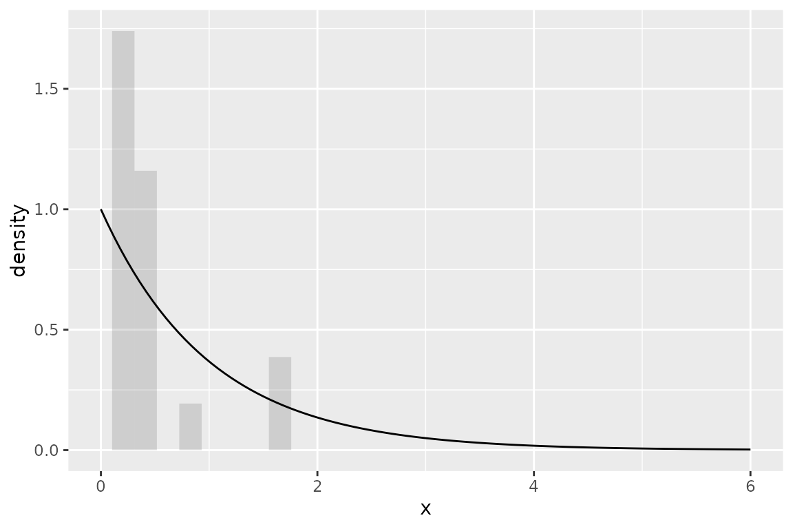
Next, we show how to estimate the rate parameter \(\lambda\) of the exponential distribution.
Maximum likelihood estimation
The MLE is the value of \(\lambda\) that maximizes the likelihood function \[ L(\lambda) = \prod_{i=1}^n f(x_i;\lambda). \] We normally work with the log-likelihood function instead of the likelihood function. Since the log-likelihood function is a monotone increasing function, the MLE is the value of \(\lambda\) that maximizes the log-likelihood function, \[ \ell(\lambda) = \sum_{i=1}^n \log f(x_i;\lambda) = \sum_{i=1}^n \bigl\{ \log \lambda - \lambda x_i \bigr\}. \]
To find the value that maximizes \(\ell\), we take the derivative of \(\ell\) with respect to \(\lambda\) and set it equal to zero. We obtain the following equation: \[ \frac{n}{\lambda} - \sum_{i=1}^n x_i = 0. \] This equation has a unique solution, \[ \hat\lambda = \frac{n}{\sum_i x_i} = \frac{1}{\bar x}, \] which is the MLE of \(\lambda\).
The algebraic.mle package provides a function mle_exp that computes the MLE of the rate parameter \(\lambda\) of the exponential distribution. Since mle_exp returns an mle object, we can use various methods and functions on it, like the summary function, to help us understand the MLE point estimate and its sampling distribution.
We can compute the MLE of the rate parameter \(\lambda\) of the exponential distribution with:
rate.hat <- mle_exp(x$x)Here is how to get a summary of the MLE:
summary(rate.hat)
#> Maximum likelihood estimator of type mle_exp is normally distributed.
#> The estimates of the parameters are given by:
#>     rate
#> 2.896701
#> The standard error is  0.5793401 .
#> The asymptotic 95% confidence interval of the parameters are given by:
#>          2.5%  97.5%
#> rate 1.701001 4.0924
#> The MSE of the estimator is  0.3502025 .
#> The MSE of the estimator is  0.3502025 .
#> The log-likelihood is  1.589309 .
#> The AIC is  -1.178618 .
The MLE of the rate parameter \(\lambda\) of the exponential distribution is \(\hat\lambda=2.8967006\), which may be computed with the point function:
point(rate.hat)
#>     rate
#> 2.896701
In the next section, we show how to estimate the sampling distribution of the MLE \(\hat\lambda\). We also show how to compute the performance measures of the MLE.
Sampling distribution of the MLE
In general, to estimate the sampling distribution, we generate \(B=10000\) samples (of size \(25\)) and their corresponding estimators, \(\hat\theta^{(1)},\ldots,\hat\theta^{(B)}\).
Normally, we do not have \(B\) samples, and if we did, we would gather all \(B\) samples into one sample (or used a weighted MLE), which would contain more (Fisher) information about \(\theta\).
However, a nice property of MLEs is that, asymptotically, they converge to a normal distribution with a mean given by the true parameter, in this case \(\lambda\), and a variance-covariance given by the inverse of the Fisher information matrix \(I\), in this case \(I(\lambda) = n/\lambda^2\), i.e., \(\hat\lambda \sim N(\lambda,I^{-1}(\lambda))\).
Next, we plot the respective densities of the non-asymptotic sampling distribution of \(\hat\theta\) and the theoretical asymptotic distribution. 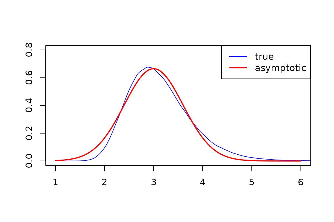
This is a relatively small sample for the MLE, but we see that the asymptotic distribution is still a good approximation.
We do not know \(\lambda\), but we may estimate it from a sample, and thus we may approximate the sampling distribution of \(\hat\lambda\) with \(N(\hat\lambda,I^{-1}(\hat\lambda))\).
We can compute the Fisher information and variance-covariance matrices with:
NOTE: If
rate.hathad been a vector,vcovwould have returned a matrix of variances and covariances, with the variances on the diagonal. (We may consider the above \(1 \times 1\) matrices.)
Since we are only giving one sample, we cannot do as we did before to provide \(B\) estimates of \(\lambda\). However, we can sample from the approximation of the asymptotic distribution of \(\hat\lambda\) with:
data.approx <- sampler(rate.hat)(B)Next, we plot the densities of the asymptotic sampling distribution and the approximation of the asymptotic sampling distribution. 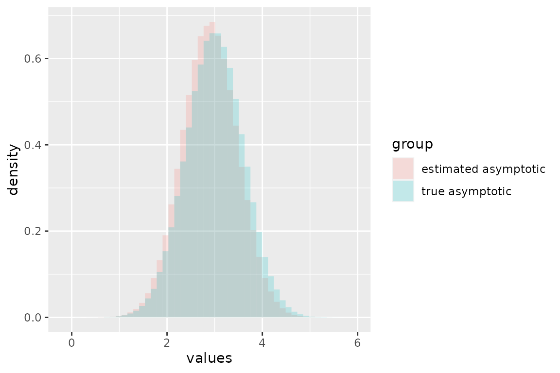
Due to sampling error, we see that the approximation, the estimate of the asymptotic sampling distribution \(N(\hat\lambda,\hat\lambda/n^{1/2})\), is shifted to the left of the sample from the true distribution, but they appear to be quite similar otherwise.
Performance measures of the MLE
We can show the confidence interval with:
confint(rate.hat)
#>          2.5%  97.5%
#> rate 1.701001 4.0924
The smaller the confidence interval, the better the estimator.
The bias \(b(\hat\lambda,\lambda) = E(\hat\lambda) - \lambda\) is another way of measuring the performance of an estimator. Ideally, the bias is zero for all components being estimated. In the MLE, the bias is asymptotically zero, but for small samples may be quite biased.
For the exponential distribution’s rate parameter, the MLE is biased. Here’s R code to compute an estimate of the bias of \(\hat\lambda\) and and the true bias of \(\hat\lambda\):
In this, they are similar.
The mean squared error (MSE) is another performance measure of an estimator. It is given by \[ \operatorname{mse}(\hat\lambda) = E\bigl\{(\hat\lambda - \lambda)^2)\bigr\}, \] which is not the same as the variance \[ \operatorname{var}(\hat\lambda) = E\bigl\{(\hat\lambda - E(\hat\lambda))^2)\bigr\}, \] since the variance only accounts for the estimators spread around its central tendency (which may be biased). Another way to compute the MSE is given by \[ \operatorname{mse}(\hat\lambda) = \operatorname{var}(\hat\lambda) + \operatorname{bias}(\hat\lambda,\lambda)^2. \] We may, of course, have to estimate the MSE if the \(\lambda\) is not known by replacing the bias with an estimate of the bias, as discussed previously.
Here’s R code to compute the MSE of \(\hat\lambda\), an estimate of the MSE and the true MSE:
They are quite similar in this case.
Prediction intervals
Frequently, we are actually interested in predicting the outcome of the random variable (or vector) that we are estimating the parameters of.
We observed a sample \(\mathcal{D} = \{T_i\}_{i=1}^n\) where \(T_i \sim \operatorname{EXP}(\lambda)\), \(\lambda\) not known. To estimate \(\lambda\), we derive the MLE \[ \hat\lambda = \frac{1}{\bar{\mathcal{D}}}, \] which, asymptotically, is normally distributed with a mean \(\lambda\) and a variance \(\lambda^2/n\).
We wish to model the uncertainty of a new observation, \(\hat{T}_{n+1}|\mathcal{D}\). We do so by considering both the uncertainty inherent to the exponential distribution and the uncertainty of our estimate \(\hat\lambda\) of \(\lambda\). In particular, we let \(\hat{T}_{n+1}|\hat\lambda \sim \operatorname{EXP}(\hat\lambda)\) and \(\hat\lambda \sim N(\lambda,\lambda^2/n)\) (the sampling distribution of the MLE). Then, the joint distribution of \(\hat{T}_{n+1}\) and \(\hat\lambda\) has the pdf given by \[ f(t,\lambda) = f_{\hat{T}|\hat\lambda}(t|\lambda) f_{\hat\lambda}(\lambda), \] and thus to find \(f(t)\), we marginalize over \(\lambda\), obtaining \[ f(t) = \int_{-\infty}^{\infty} f_{\hat{T}_{n+1},\hat\lambda}(t,r) dr. \]
Given the information in the sample, the uncertainty in the new observation is characterized by the distribution \[ \hat{T}_{n+1} \sim f(t). \]
It has greater variance than \(T_{n+1}|\hat\lambda \sim \operatorname{EXP}(\hat\lambda)\) because, as stated earlier, we do not know \(\lambda\), we only have an uncertain estimate \(\hat\lambda\).
In pred, we compute the predictive interval (PI) of the distribution of \(\hat{T}_{n+1}\) using Monte Carlo simulation, where we replace the integral with a sum over a large number of draws from the joint distribution of \(\hat{T}_{n+1}\) and \(\hat\lambda\) and then compute the empirical quantiles.
The function pred takes as arguments x, in this case an mle object, and a sampler for the distribution of the random variable of interest, in this case rexp (the sampler for the exponential distribution). The sampler must be compatible with the parameter value of x (i.e., point(x)). Here is how we compute the PI for \(\hat{T}_{n+1}\):
rate.hat <- mle_exp(rexp(n,rate))
pred(x=rate.hat,samp=rexp)
#>           mean      lower    upper
#> [1,] 0.2905545 0.00711804 1.117284
How does this compare to \(T_{n+1}|\hat\lambda \sim \operatorname{EXP}(\hat\lambda = 3.5948592)\)?
q.95 <- c(1/point(rate.hat),qexp(c(.025,.975),point(rate.hat)))
names(q.95) <- c("mean","lower", "upper")
print(q.95)
#>        mean       lower       upper
#> 0.278175010 0.007042781 1.026154077
We see that the 95% quantile interval for \(T_{n+1}|\hat\lambda\) is a bit smaller than \(\hat{T}_{n+1}\), which is what we expected. Of course, for sufficiently large sample sizes, they will converge to the same quantiles.