![]()
algebraic.mle is an R package that provides an algebra
over Maximum Likelihood Estimators (MLEs). These estimators possess many
desirable, well-defined statistical properties which the package helps
you manipulate and utilize.
Installation
The R package algebraic.mle can be installed from GitHub
by using the devtools package in R:
install.packages("devtools")
devtools::install_github("queelius/algebraic.mle")
Normal distribution
We are going to the classic Normal distribution to demonstrate how to
use algebraic.mle. We are using it for a few reasons:
- It’s well-understood, so we can compare our results to the known results.
- It’s a very common distribution, so it’s useful to have a good understanding of its properties.
- The MLE is multivariate, so we can demonstrate how to use
algebraic.mlefor multivariate distributions.
So, first, we define a simple MLE solver for the normal distribution.
fit_normal <- function(data) {
    sigma <- function(data) {
        mean((data - mean(data))^2)
    }
    loglik <- function(par, data) {
        n <- length(data)
        -n / 2 * log(2 * pi * par[2]) - 1 / (2 * par[2]) *
            (sum(data^2) - 2 * par[1] * sum(data) + n * par[1]^2)
    }
    par.hat <- c(mu = mean(data), var = sigma(data))
    H <- numDeriv::hessian(func = loglik, x = par.hat, data = data)
    algebraic.mle::mle(
        theta.hat = par.hat,
        loglike = loglik(par.hat, data),
        score = numDeriv::grad(func = loglik, x = par.hat, data = data),
        sigma = MASS::ginv(-H),
        info = -H,
        obs = NULL,
        nobs = length(data),
        superclasses = c("mle_normal"))
}
As you can see, we return an mle object, and then we
give it a sub-class mle_normal (it is also a subclass of
mle and algebraic.dist’s dist) so
we can specialize some of the methods for MLE of the normal
distribution, e.g., bias.mle_normal which we show
later.
Monte-carlo (MC) simulation of the sampling distribution of the MLE
Let’s define theta_samp_mc, which stands for the Monte
Carlo simulation of the sampling distribution of the MLE. It takes a
sample size n, a true parameter value theta,
and a number of simulations B to run. It returns a matrix
with B rows and two columns, the first column is the MLE of
the mean and the second column is the MLE of the variance.
theta_samp_mc <- function(n, theta, B = 10000) {
    mu <- theta[1]
    var <- theta[2]
    mles <- matrix(NA, nrow = B, ncol = 2)
    for (i in 1:B) {
        d <- rnorm(n, mean = mu, sd = sqrt(var))
        mles[i, ] <- params(fit_normal(d))
    }
    colnames(mles) <- c("mu", "var")
    mles
}
# Set up the parameters of a simulation
set.seed(913254)
n <- 70
mu <- 1
var <- 1
B <- 1000
theta <- c(mu, var)
mles <- theta_samp_mc(n = n, theta = theta, B = B)
head(mles)
#>         mu   var
#> [1,] 0.891 0.728
#> [2,] 1.033 1.102
#> [3,] 1.105 1.094
#> [4,] 1.146 0.832
#> [5,] 0.916 0.895
#> [6,] 0.986 0.904
The matrix mles is a sample of MLEs from the sampling
distribution of the MLE. It is an empirical distribution of the
MLE
from samples of size
for
.
This particular example is Monte Carlo simulation of the sampling distribution, since we are simulating the sampling distribution by repeatedly sampling from the population distribution and computing the MLE for each sample.
In bootstrap, we would resample from the sample, not the population, but with a large enough sample, the two will produce nearly identical results. See the bootstrap section for more details, where we’ll compare the two.
For a sufficiently large number of simulations
,
the empirical sampling distribution should be very close to the true
sampling distribution. We can plot the empirical sampling distribution
of the MLEs using the plot function on the
mles matrix.
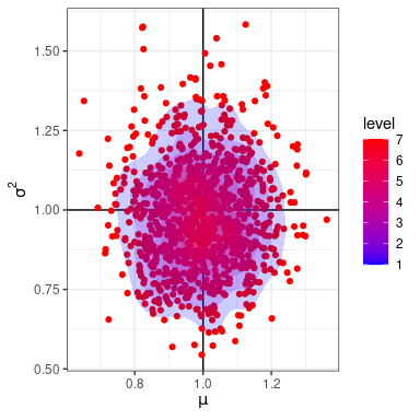
Sampling distribution of the MLEs.
In algebraic.dist, we can use
empirical_dist to represent an empirical sampling
distribution by giving it the sample of MLEs previously generated:
theta.mc <- algebraic.dist::empirical_dist(mles)In general, for any MLE and assuming the the regularity conditions hold, the asymptotic sampling distribution of the MLE is normal with mean and variance-covariance matrix , where is the Fisher information matrix and is the sample size. However, in general:
- We don’t know when the asymptotic sampling distribution is a good approximation to the true sampling distribution. In these cases, the empirical sampling distribution may be used instead.
- We may not be confident our implementation of the MLE is correct, in which case the empirical sampling distribution can be used to check our implementation.
- The regularity conditions may not hold, in which case the asymptotic sampling distribution may not be known. In these cases, the empirical sampling distribution may be used instead.
With these caveats in mind, we compare some of the statistics of the empirical sampling distribution of the MLE for the normal distribution and the asymptotic sampling distribution.
Let’s look at some basic parameters of the sampling distribution of the MLE for the normal distribution. First, let’s look at the mean:
(mu.mc <- mean(theta.mc))
#>    mu   var
#> 0.995 0.982
The mean looks pretty close to the true parameter vector
We can actually compute any parameter, since theta.mc,
models the concept of a distribution. In particular, it models a
distribution in algebraic.dist, and thus the API exposed by
algebraic.dist is available to us. For instance, we can
compute various parameters of the sampling distribution of the MLE using
the expectation function:
# should sum to 1
expectation(theta.mc, function(x) 1)
#> [1] 1
# mean
expectation(theta.mc, function(x) x)
#>    mu   var
#> 0.995 0.982
# variance of (mu, var)
expectation(theta.mc, function(x) (x - mu.mc)^2)
#>     mu    var
#> 0.0136 0.0282
# kurtosis of (mu, var)
expectation(theta.mc, function(x) (x - mu.mc)^4) /
    expectation(theta.mc, function(x) (x - mu.mc)^2)^2
#>   mu  var
#> 2.77 3.21
# skewness of mu and var -- should be (0, 0)
expectation(theta.mc, function(x) ((x - mu.mc) / theta)^3)
#>        mu       var
#> 0.0000624 0.0016654
# covariance of (mu, var) -- should be around 0
expectation(theta.mc, function(x) (x[1] - mu.mc[1]) * (x[2] - mu.mc[2]))
#> [1] 0.0000799
We could use the mean and variance-covariance matrix to parameterize a multivariate normal distribution (MVN), for instance, but we don’t do that here.
Bias
Bias is a measure of the systematic error of an estimator; it measures how far its average value is from the true value being estimated. Formally, it is defined as the difference between the expected value of the estimator and the true value of the parameter, i.e., where denotes the expectation operator with respect to the sampling distribution of . (Normally, we drop the subscript in the expectation operator and write instead of unless it’s not clear from context which expectation operator we are using.)
When the bias is zero, the estimator is unbiased, otherwise
it is biased. Analytically, the asymptotic bias of the MLE for
the parameters of the normal distribution is
Plugging in the true value of
and the sample size
,
we get
.
We may also provide an appropriate implementation of the
bias method in algebraic.mle for
mle_normal (which is what we called our the object that we
returned from fit_normal):
bias.mle_normal <- function(x, par = NULL, ...) {
    if (is.null(par)) {
        par <- params(x)
    }
    c(mu = 0, var = -(1 / nobs(x)) * par[2])
}
Now, let’s compute the bias using this function, and the estimate of
the bias provided by the bias.mle_emp:
# first, we sample some data from the true distribution
data <- rnorm(n = n, mean = mu, sd = sqrt(var))
# now we fit it to the normal distribution
theta.hat <- fit_normal(data)
# now we compute the bias, first using the asymptotic theory
bias(theta.hat, theta)
#> mu var
#> 0.0000 -0.0143
# now using the empirical sampling distribution
expectation(theta.mc, function(x) x - theta) # mean(theta.mc) - theta
#> mu var
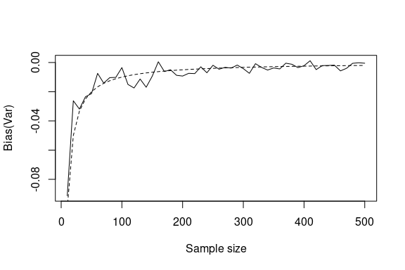
#> -0.00507 -0.01768The asymptotic bias and the empirical bias are pretty close. Let’s see how the bias of the variance changes as the sample size increases.
N <- 1000
ns <- seq(10, 500, 10)
bias_var <- numeric(length(ns))
j <- 1
for (n in ns) {
    vars <- numeric(length(N))
    for (i in 1:N) {
        d <- rnorm(n = n, mean = mu, sd = sqrt(var))
        fit <- fit_normal(d)
        vars[i] <- params(fit)[2]
    }
    bias_var[j] <- mean(vars) - var
    j <- j + 1
}
Variance-covariance matrix
The variance-covariance matrix is one of the more important statistical measures of an estimator of a parameter vector. It quantities both the variability of the individual parameter estimates and how they co-vary with each other.
The variance-covariance matrix of a parameter vector is an matrix defined as
The th element of the variance-covariance matrix is the covariance between the th and th elements of the parameter vector, respectively and . Thus, the diagonal elements of the variance-covariance matrix are the variances of the individual parameter estimates, and the off-diagonal elements are the covariances between the parameter estimates.
round(vcov(theta.hat), digits=3)
#>       [,1]  [,2]
#> [1,] 0.011 0.000
#> [2,] 0.000 0.017
round(vcov(theta.mc), digits=3)
#>        mu   var
#> mu  0.014 0.000
#> var 0.000 0.028
They look reasonably close, suggesting at , the asymptotic sampling distribution is a good approximation to the “true” sampling distribution of the MLE.
Confidence intervals
We can compute the CI of a parameter using the confint
function:
confint(theta.hat)
#> 2.5% 97.5%
#> mu 0.724 1.14
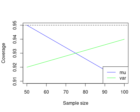
#> var 0.522 1.04A very important measure of the accuracy of an estimator is its coverage probability, which is the probability that the confidence interval for the parameter estimate contains the true value of the parameter. If the coverage probability for an -confidence interval is , then the confidence interval is said to be well-calibrated. If the coverage probability is less than , then the confidence interval is said to be conservative; if the coverage probability is greater than , then the confidence interval is said to be anti-conservative.
We can estimate it by simulating a large number of samples from the population distribution and computing the proportion of times the confidence interval contains the true value of the parameter. We can do this for both the mean and variance of the normal distribution.
Click to show/hide R code
N <- 1000
ns <- c(seq(50, 200, 50), 300, 600, 1000)
coverage_prob <- matrix(NA, nrow=length(ns), ncol=2)
j <- 1
for (n in ns) {
    count1 <- 0L
    count2 <- 0L
    for (i in 1:N) {
        d <- rnorm(n = n, mean = mu, sd = sqrt(var))
        fit <- fit_normal(d)
        ci <- confint(fit)
        if (ci[1, 1] <= mu && mu <= ci[1, 2]) {
            count1 <- count1 + 1
        }
        if (ci[2, 1] <= var && var <= ci[2, 2]) {
            count2 <- count2 + 1
        }
    }
    coverage_prob[j, 1] <- count1 / N
    coverage_prob[j, 2] <- count2 / N
    j <- j + 1
}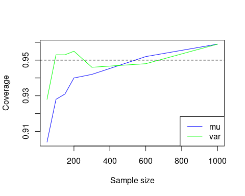
We see that the coverage probability is close to the nominal coverage probability, and converges to it as the sample size increases. This suggests that the confidence intervals are well-calibrated.
Mean squared error matrix
The mean squared error (MSE) of an estimator of a parameter vector is defined as where is a column vector of differences between the estimator and the true parameter and is a row vector of the same differences, and we are performing a standard matrix multiplication between the two vectors. The MSE is a measure of the average squared error of the estimator. It is a function of the true parameter value .
This MSE is a matrix. It is very similar to the variance-covariance matrix, which is defined as where we replace the true paramater with the expected value of the estimator . If the estimator is unbiased, then and .
We not only need to consider the estimation error for each parameter individually, but also how these errors might relate to each other. For instance, it could be the case that when we overestimate one parameter, we tend to underestimate another. This kind of relationship between errors in estimating different parameters can be captured by the off-diagonal elements of the MSE matrix, which represent the covariances between errors.
The diagonal elements of the MSE represent the MSE of the individual parameter estimators, e.g., the th diagonal element represents .
The trace of the MSE, the sum of the diagonal elements, represents the total MSE across all parameters. As a single summary statistic, it may be useful for comparing different estimators.
The MSE can be decomposed into two parts:
- The bias, which is the difference between the expected value of the estimator and the true parameter value, and
- The variance, which is the variance of the estimator.
The MSE is then computed as the sum of the bias outer product and the variance-covariance matrix:
mse.hat <- mse(theta.hat, theta)
mse.mc <- matrix(expectation(theta.mc,
    function(x) (x - theta) %*% t(x - theta)), nrow = 2)

round(mse.hat, digits = 3)
#>         mu   var
#> [1,] 0.011 0.000
#> [2,] 0.000 0.018
round(mse.mc, digits = 3)
#>       [,1]  [,2]
#> [1,] 0.014 0.000
#> [2,] 0.000 0.029
It’s hard to distinguish the MSE matrices from the variance-covariance matrices reported previously, which is not surprising, since the bias is relatively small and so the MSE is dominated by the variance.
Let’s take a closer look at the variance and MSE of the mean :
# temporarily show more digits in the numbers/outputs for this code block
op <- options(digits = 12)
# mse(mu)
expectation(theta.mc, function(x) (x[1] - mu)^2)
#> [1] 0.013651619343
# variance(mu)
(mu.var <- expectation(theta.mc, function(x) (x[1] - mean(theta.mc)[1])^2))
#> [1] 0.013625962941
b <- expectation(theta.mc, function(x) x[1] - mu)
# mse = bias^2 + variance
b^2 + mu.var
#> [1] 0.013651619343
options(op)
They are very close, since the bias is so small.
We should take the MSE from the Monte Carlo simulation as a sort of
“true” MSE, since it is computed from the empirical sampling
distribution of the MLE. We expect that as the sample size increases,
the asymptotic MSE (mse.hat) and the MC MSE
(mse.mc) will converge to the same value. In fact, let’s
run a little experiment to show this:
ns <- seq(25, 200, 25)
mses.mc <- matrix(NA, nrow = length(ns), ncol = 2)
mses.hat <- matrix(NA, nrow = length(ns), ncol = 2)
mses.hat.hat <- matrix(NA, nrow = length(ns), ncol = 2)
j <- 1
for (n in ns) {
    theta.n <- empirical_dist(theta_samp_mc(n = n, theta = theta, B = B))
    # Use mean() on the sampled distribution for MSE calculation
    samples <- obs(theta.n)
    mse.mu.n <- mean((samples[, 1] - mu)^2)
    mse.var.n <- mean((samples[, 2] - var)^2)
    data <- rnorm(n = n, mean = mu, sd = sqrt(var))
    fit <- fit_normal(data)
    mses.mc[j, ] <- c(mse.mu.n, mse.var.n)
    mses.hat[j, ] <- diag(mse(fit, theta))
    mses.hat.hat[j, ] <- diag(mse(fit))
    j <- j + 1
}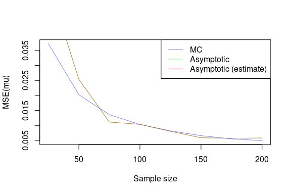
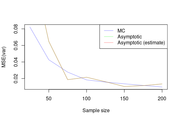
These plots demonstrate that the asymptotic MSE is a good approximation to the “true” MSE, which is the MSE computed from the empirical sampling distribution of the MLE.
It’s difficult to distinguish the estimated asymptotic MSE, where the true parameter is not known, from the asymptotic MSE, where the true parameter is known. This is because the bias is so small, and so the MSE is dominated by the variance.
Bootstrap of the sampling distribution of the MLE
Normally, we don’t know the true data generating process (DGP) of the data we observe. We only have a sample of data, and we want to use that sample to estimate the parameters of some model that hopefully provides a good fit to the DGP using maximum likelihood estimation.
Earlier, we simulated a sample of data from a normal distribution with mean 1 and variance 1 and then used MLE on each sample to generate an empirical sampling distribution of the MLE. This is called Monte Carlo simulation.
However, we can also use the sample of data we have to generate an empirical sampling distribution of the MLE. This is called bootstrap. The idea is that the sample we have is a sample from the true DGP, and we can use that sample to generate new samples (resample) and fit an MLE to each of these to generate an Bootstrapped empirical sampling distribution of the MLE.
# Simulate a sample of n observations from a normal with mean 1 and variance 2.
library(boot)
theta.boot <- mle_boot(boot(
    data = data,
    statistic = function(x, ind) {
        params(fit_normal(x[ind]))
    },
    R = B))
Let’s compute some statistics:
params(theta.boot)
#>   mu  var
#> 1.09 1.01
confint(theta.boot)
#>      2.5% 97.5%
#> mu  0.952  1.22
#> var 0.825  1.20
Let’s use these Bootstrapped MLEs to generate an aproximation of the empirical sampling distribution:
theta.b <- empirical_dist(theta.boot$t)As before, let’s do some basic expectations of the Bootstrapped sampling distribution of the MLE and compare to the previous results:
# should sum to 1
expectation(theta.b, function(x) 1)
#> [1] 1
# mean
(mu.b <- mean(theta.b))
#> [1] 1.08 1.01
# variance of (mu, var)
expectation(theta.b, function(x) (x - mu.b)^2)
#> [1] 0.00471 0.00937
# kurtosis of (mu, var)
expectation(theta.b, function(x) (x - mu.b)^4) /
    expectation(theta.b, function(x) (x - mu.b)^2)^2
#> [1] 2.84 2.91
# skewness of mu and var -- should be (0, 0)
expectation(theta.b, function(x) ((x - mu.b) / theta)^3)
#> [1] 0.0000123 0.0001203
# covariance of (mu, var) -- should be around 0
expectation(theta.b, function(x) (x[1] - mu.b[1]) * (x[2] - mu.b[2]))
#> [1] 0.000795
These are not too bad.
Let’s compute the bias and compare it to the previous results:
bias(theta.boot)
#>       mu      var
#> -0.00144 -0.00459
expectation(theta.mc, function(x) x - theta)
#>       mu      var
#> -0.00507 -0.01768
bias(theta.hat, theta)
#>      mu     var
#>  0.0000 -0.0143
We see that the bias function for mle_boot
is not too bad. Note that the bias is an expectation w.r.t.
the sampling distribution of the MLE. In general, we can have a better
estimator if we use
assuming the bias estimate is accurate.
In this particular example that transformation makes it worse, which is
fine, the bias of the transformed estimator would be less in theory.
Howevever, in practice, we don’t trust the bias reported by the
Bootstrap, except as evidence that our estimator is biased or not. The
analytic bias, bias.mle_normal, is more accurate, and will
generally produce estimators with less bias (although by the
bias-variance trade-off, it may have more variance).
Let’s compare the variance-covariance matrix of the Bootstrapped sampling distribution of the MLE to the “true” sampling distribution and the asymptotic sampling distribution:
round(vcov(theta.b), digits = 3)
#>       [,1]  [,2]
#> [1,] 0.005 0.001
#> [2,] 0.001 0.009
round(vcov(theta.mc), digits = 3)
#>        mu   var
#> mu  0.014 0.000
#> var 0.000 0.028
round(vcov(theta.hat), digits = 3)
#>       [,1]  [,2]
#> [1,] 0.011 0.000
#> [2,] 0.000 0.017Click to show/hide R code
N <- 100
ns <- c(50, 100)
coverage_prob <- matrix(NA, nrow=length(ns), ncol=2)
j <- 1
for (n in ns) {
    count1 <- 0L
    count2 <- 0L
    for (i in 1:N) {
        d <- rnorm(n = n, mean = mu, sd = sqrt(var))
        fit.boot <- mle_boot(boot(
            data = d,
            statistic = function(x, ind) {
                params(fit_normal(x[ind]))
            },
            R = 250))
        ci <- confint(fit.boot)
        if (ci[1, 1] <= mu && mu <= ci[1, 2]) {
            count1 <- count1 + 1
        }
        if (ci[2, 1] <= var && var <= ci[2, 2]) {
            count2 <- count2 + 1
        }
    }
    coverage_prob[j, 1] <- count1 / N
    coverage_prob[j, 2] <- count2 / N
    #cat("n = ", n, ", coverage = ", coverage_prob[j, ], "\n")
    j <- j + 1
}
Prediction intervals
Frequently, we are actually interested in predicting the outcome of the random variable (or vector) that we are estimating the parameters of.
We observed a sample where , not known. To estimate , we solved the MLE which, asymptotically, is normally distributed with a mean and a variance-covariance given by the inverse of the FIM (or, using the Bootstrap, by estimating the covariance of the sampling distribution of the Bootstrapped MLEs).
We wish to model the uncertainty of a new observation, . We do so by considering both the uncertainty inherent to the Normal distribution and the uncertainty of our estimate . In particular, we let and . Then, the joint distribution of and has the pdf given by and thus to find , we marginalize over , obtaining
Given the information in the sample, the uncertainty in the new observation is characterized by the distribution
It has greater variance than because, as stated earlier, we do not know , we only have an uncertain estimate .
In pred, we compute the predictive interval (PI) of the
distribution of
using Monte Carlo integration, i.e., sum over a large number of draws
from the joint distribution of
and
and then compute the empirical quantiles.
The function pred takes as arguments x, in
this case an mle object, and a sampler for the distribution
of the random variable of interest, in this case rnorm (the
sampler for the normal distribution). The sampler must be compatible
with the parameter value of x (i.e.,
params(x)). Here is how we compute the PI for
:
samp <- function(n, par) rnorm(n = n, mean = par[1], sd = sqrt(par[2]))
pred(x = theta.hat, samp = samp)
#>       mean  lower upper
#> [1,] 0.933 -0.824   2.7
How does this compare to ?
par <- params(theta.hat)
mu.hat <- par[1]
var.hat <- par[2]
c(mu.hat, qnorm(c(.025,.975), mean = mu.hat, sd = sqrt(var.hat)))
#>     mu
#>  0.931 -0.801  2.663
We see that the 95% quantile interval for is a bit smaller than , which is what we expected. Of course, for sufficiently large sample sizes, they will converge to the same quantiles.
Weighted MLE: a weighted sum of maximum likelihood estimators
Since the variance-covariance of an MLE is inversely proportional to the FIM that the MLE is defined with respect to, we can combine multiple MLEs of , each of which may be defined with respect to a different kind of sample, to arrive at the MLE that incorporates the Fisher information in all of those samples.
Consider mutually independent MLEs of parameter , , where . Then, the sampling MLE of that incorporates all of the data in is given by the inverse-variance weighted mean, which, asymptotically, has an expected value of and a variance-covariance of .
To evaluate the performance of the weighted MLE, we generate a sample of observations from and compute the MLE for the observed sample, denoted by .
We then divide the observed sample into sub-samples, each of size , and compute the MLE for each sub-sampled, denoted by .
Finally, we do a weighted combination these MLEs to form the weighted MLE, denoted by :
N <- 100
r <- 5
samp <- rnorm(N, mean = theta[1], sd = sqrt(theta[2]))
samp.sub <- matrix(samp, nrow = r)
mles.sub <- list(length = r)
for (i in 1:r)
    mles.sub[[i]] <- fit_normal(samp.sub[i,])

mle.wt <- mle_weighted(mles.sub)
mle <- fit_normal(samp)
We show the results in the following R code. First, we show the weighted MLE and its MSE:
params(mle.wt)
#> [1] 1.221 0.778
vcov(mle.wt)
#>                    [,1]               [,2]
#> [1,] 0.0080147769950214 0.0000000000000257
#> [2,] 0.0000000000000257 0.0124697701682341
The MLE for the total sample and its MSE is:
params(mle)
#>    mu   var
#> 1.210 0.864
vcov(mle)
#>                    [,1]               [,2]
#> [1,] 0.0086408549278714 0.0000000000000244
#> [2,] 0.0000000000000244 0.0149328747769700
Unfortuantely, is a much better estimator of than . According to theory, they should be identical, but in practice, there may be issues like numerical instability that cause the weighted MLE to perform poorly.
We are in fact using numerical differentiation to compute the FIM, which may be a source of error. We can try to improve the accuracy of the FIM by using a more accurate method of computing the FIM, such as an analytical solution or a more accurate numerical approximation.