flexhaz: Hazard-First Survival Modeling

The Problem

Standard parametric survival models force you to choose from a short list of hazard shapes: constant (exponential), monotone power-law (Weibull), exponential growth (Gompertz). But real failure patterns rarely cooperate:

• Ceramic capacitors exhibit wear-out that accelerates with age — the failure rate climbs faster than any power law.
• Software systems follow a bathtub curve: early crashes from latent bugs, a stable period, then increasing failures as dependencies rot.
• Post-surgical patients face high initial risk that drops sharply, then slowly rises again as long-term complications emerge.

Each of these demands a hazard function that standard families cannot express. You can reach for semi-parametric methods (Cox regression), but then you lose the ability to extrapolate, simulate, or compute closed-form quantities like mean time to failure.

The Idea

flexhaz takes a different approach: you write the hazard function, and the package derives everything else.

Given a hazard (failure rate) function $h(t)$, the full distribution follows:

$$h(t) \;\xrightarrow{\;\int\;}\; H(t) = \int_0^t h(u)\,du \;\xrightarrow{\;\exp\;}\; S(t) = e^{-H(t)} \;\xrightarrow{\;\times h\;}\; f(t) = h(t)\,S(t)$$

If you can express $h(t)$ as an R function of time and parameters, flexhaz gives you survival curves, CDFs, densities, quantiles, random sampling, log-likelihoods, MLE fitting, and residual diagnostics — automatically.

Installation

# From r-universe
install.packages("flexhaz", repos = "https://queelius.r-universe.dev")

Your First Distribution

library(flexhaz)

Let’s start with the simplest case: the exponential distribution with constant failure rate.

# Exponential with failure rate lambda = 0.1 (MTTF = 10 time units)
exp_dist <- dfr_exponential(lambda = 0.1)
print(exp_dist)
#> Dynamic failure rate (DFR) distribution with failure rate:
#> function (t, par, ...) 
#> {
#>     rep(par[[1]], length(t))
#> }
#> <bytecode: 0x55a740bc6348>
#> <environment: 0x55a740bc86c8>
#> It has a survival function given by:
#>     S(t|rate) = exp(-H(t,...))
#> where H(t,...) is the cumulative hazard function.

Get Distribution Functions

All distribution functions follow a two-step pattern — the method returns a closure that you then call with time values:

# Get closures
S <- surv(exp_dist)
h <- hazard(exp_dist)
f <- density(exp_dist)

# Evaluate at specific times
S(10)   # P(survive past t=10) = exp(-0.1 * 10) ~ 0.37
#> [1] 0.3678794
h(10)   # Hazard at t=10 = 0.1 (constant for exponential)
#> [1] 0.1
f(10)   # PDF at t=10
#> [1] 0.03678794

You can verify these analytically: $S(10) = e^{-0.1 \times 10} = e^{-1} \approx 0.368$, the hazard is constant at $\lambda = 0.1$, and $f(10) = \lambda \, S(10) = 0.1 \times 0.368 \approx 0.0368$.

Generate Samples

samp <- sampler(exp_dist)
set.seed(42)
failure_times <- samp(20)

# Sample mean should be close to MTTF = 1/lambda = 10
mean(failure_times)
#> [1] 13.31295

With only 20 samples the mean can deviate noticeably from the theoretical MTTF of 10. Larger samples converge closer.

Fitting to Data

Now let’s fit a model to survival data using maximum likelihood estimation.

set.seed(123)
n <- 50
df <- data.frame(
  t = rexp(n, rate = 0.08),   # True lambda = 0.08
  delta = rep(1, n)            # All exact observations
)
head(df)
#>            t delta
#> 1 10.5432158     1
#> 2  7.2076284     1
#> 3 16.6131858     1
#> 4  0.3947170     1
#> 5  0.7026372     1
#> 6  3.9562652     1

Maximum Likelihood Estimation

# Template with no parameters (to be estimated)
exp_template <- dfr_exponential()

solver <- fit(exp_template)
result <- solver(df, par = c(0.1))  # Initial guess
coef(result)
#> [1] 0.07077333

# Compare to analytical MLE: lambda_hat = n / sum(t)
n / sum(df$t)
#> [1] 0.07077323

The numerical MLE matches the closed-form solution $\hat\lambda = n / \sum t_i$ to five decimal places. Both estimate $\lambda \approx 0.071$, which is consistent with the true value of 0.08 given the sampling variability at $n = 50$.

Model Diagnostics

Check model fit using Cox-Snell residuals (should follow the Exp(1) diagonal):

fitted_dist <- dfr_exponential(lambda = coef(result))
qqplot_residuals(fitted_dist, df)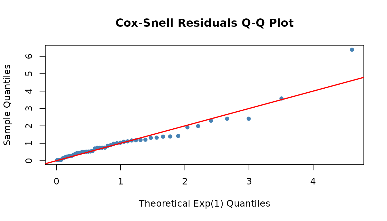

Working with Censored Data

Real survival data often includes censoring — observations where the exact failure time is not directly observed. The flexhaz package uses a delta column to encode three types of observation:

delta	Meaning	Log-likelihood contribution
1	Exact failure	$\log h(t) - H(t)$
0	Right-censored (survived past $t$)	$-H(t)$
-1	Left-censored (failed before $t$)	$\log(1 - e^{-H(t)})$

Right-Censoring

Right-censoring is the most common type — the subject was still alive (or the device was still running) when observation ended.

df_censored <- data.frame(
  t = c(5, 8, 12, 15, 20, 25, 30, 30, 30, 30),
  delta = c(1, 1, 1, 1, 1, 0, 0, 0, 0, 0)  # Last 5 right-censored at t=30
)

solver <- fit(dfr_exponential())
result <- solver(df_censored, par = c(0.1))
coef(result)
#> [1] 0.02439454

The censored MLE properly accounts for the five units that survived past $t = 30$. You can verify: the analytical MLE for censored exponential data is $\hat\lambda = d / \sum t_i$ where $d$ is the number of failures, giving $5 / 205 \approx 0.024$ — exactly what the optimizer returns.

Left-Censoring

Left-censoring arises when we know failure occurred before an inspection time, but not exactly when. This is common in periodic-inspection studies: you check a device at time $t$ and discover it has already failed.

df_left <- data.frame(
  t = c(5, 10, 15, 20),
  delta = c(-1, -1, 1, 0)   # left-censored, left-censored, exact, right-censored
)

solver <- fit(dfr_exponential())
result <- solver(df_left, par = c(0.1))
coef(result)
#> [1] 0.07184419

This dataset mixes all three observation types: two left-censored, one exact failure at $t = 15$, and one right-censored at $t = 20$. The estimate $\hat\lambda \approx 0.072$ is higher than a right-censored-only estimate because the left-censored observations provide evidence of earlier failures. All three types can coexist in the same dataset — the log-likelihood sums the appropriate contribution for each observation.

Custom Column Names

By default, flexhaz looks for columns named t (observation time) and delta (event indicator). When your data uses different column names — as is common with clinical datasets — use the ob_col and delta_col arguments:

clinical_data <- data.frame(
  time = c(5, 8, 12, 15, 20),
  status = c(1, 1, 1, 0, 0)
)

dist <- dfr_exponential()
dist$ob_col <- "time"
dist$delta_col <- "status"

solver <- fit(dist)
result <- solver(clinical_data, par = c(0.1))
coef(result)
#> [1] 0.05

The estimate $\hat\lambda = 0.05$ equals $3 / 60 = d / \sum t_i$, confirming that the column mapping works correctly.

You can also set custom columns at construction time via dfr_dist():

dist <- dfr_dist(
  rate = function(t, par, ...) rep(par[1], length(t)),
  cum_haz_rate = function(t, par, ...) par[1] * t,
  ob_col = "time",
  delta_col = "status"
)

Beyond Exponential: Weibull

The exponential assumes constant failure rate. For increasing or decreasing failure rates, use Weibull:

# Weibull with increasing failure rate (wear-out)
weib_dist <- dfr_weibull(shape = 2, scale = 20)

# Compare hazard functions
plot(weib_dist, what = "hazard", xlim = c(0, 30), col = "blue",
     main = "Hazard Comparison")
plot(dfr_exponential(lambda = 0.05), what = "hazard", add = TRUE, col = "red")
legend("topleft", c("Weibull (shape=2)", "Exponential"),
       col = c("blue", "red"), lwd = 2)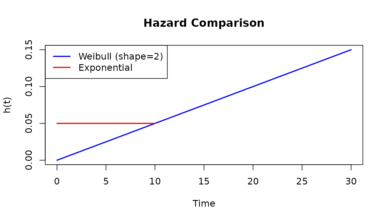

Weibull shape parameter interpretation:

• shape < 1: Decreasing hazard (infant mortality, burn-in failures)
• shape = 1: Constant hazard (exponential)
• shape > 1: Increasing hazard (wear-out, aging)

The Real Power: Custom Hazards

Where flexhaz truly shines is modeling non-standard hazard patterns that no built-in distribution can express.

Define a bathtub hazard

$$h(t) = a\,e^{-bt} + c + d\,t^k$$

Three additive components: exponential decay (infant mortality), constant baseline (useful life), and power-law growth (wear-out).

bathtub <- dfr_dist(
  rate = function(t, par, ...) {
    a <- par[[1]]  # infant mortality magnitude
    b <- par[[2]]  # infant mortality decay
    c <- par[[3]]  # baseline hazard
    d <- par[[4]]  # wear-out coefficient
    k <- par[[5]]  # wear-out exponent
    a * exp(-b * t) + c + d * t^k
  },
  par = c(a = 0.5, b = 0.5, c = 0.01, d = 5e-5, k = 2.5)
)

Plot the hazard curve

h <- hazard(bathtub)
t_seq <- seq(0.01, 30, length.out = 300)
plot(t_seq, sapply(t_seq, h), type = "l", lwd = 2, col = "darkred",
     xlab = "Time", ylab = "Hazard rate h(t)",
     main = "Bathtub Hazard Function")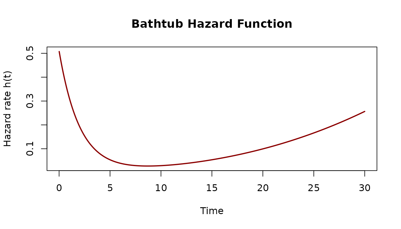

Plot the survival curve

plot(bathtub, what = "survival", xlim = c(0, 30),
     col = "darkblue", lwd = 2,
     main = "Survival Function S(t)")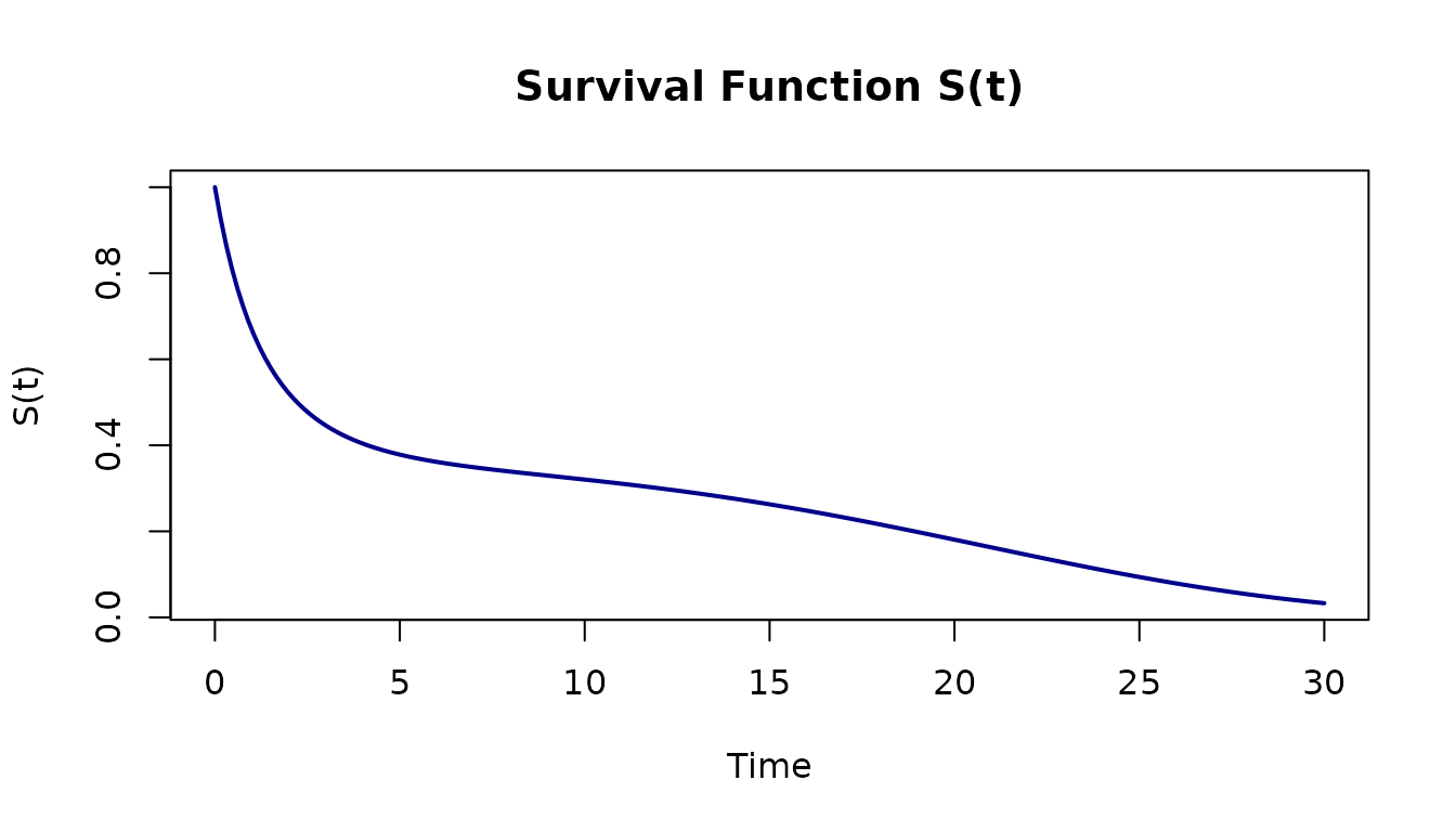

Simulate data and fit via MLE

# Generate failure times, right-censored at t = 25
set.seed(42)
samp <- sampler(bathtub)
raw_times <- samp(80)
censor_time <- 25

df <- data.frame(
  t = pmin(raw_times, censor_time),
  delta = as.integer(raw_times <= censor_time)
)

cat("Observed failures:", sum(df$delta), "out of", nrow(df), "\n")
#> Observed failures: 68 out of 80
cat("Right-censored:", sum(1 - df$delta), "\n")
#> Right-censored: 12

# Fit the model
solver <- fit(bathtub)
result <- solver(df,
  par = c(0.3, 0.3, 0.02, 1e-4, 2),
  method = "Nelder-Mead"
)

Inspect the fit

cat("Estimated parameters:\n")
#> Estimated parameters:
print(coef(result))
#> [1] 0.4828059584 0.6478481588 0.0128496924 0.0003329348 1.7388288598

cat("\nTrue parameters:\n")
#> 
#> True parameters:
print(c(a = 0.5, b = 0.5, c = 0.01, d = 5e-5, k = 2.5))
#>       a       b       c       d       k 
#> 0.50000 0.50000 0.01000 0.00005 2.50000

With five parameters and only 80 observations, the optimizer recovers the general shape but not every parameter exactly. In particular, $d$ and $k$ trade off: a smaller exponent with a larger coefficient can produce a similar wear-out curve. The Q-Q plot below is the real test of fit quality.

Residual diagnostics

fitted_bathtub <- dfr_dist(
  rate = function(t, par, ...) {
    par[[1]] * exp(-par[[2]] * t) + par[[3]] + par[[4]] * t^par[[5]]
  },
  par = coef(result)
)
qqplot_residuals(fitted_bathtub, df)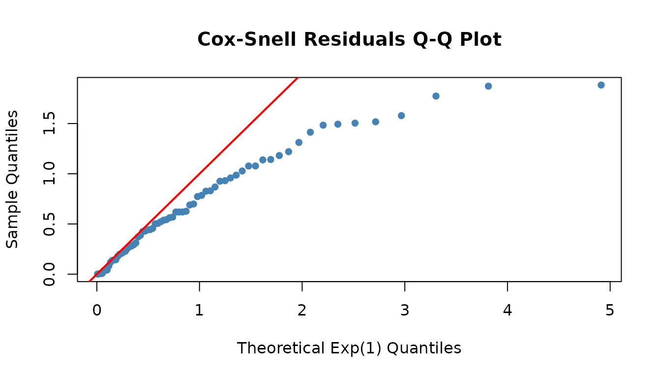

Points near the diagonal indicate the model captures the failure pattern well.

Built-in Distributions

For common parametric families, the package provides optimized constructors with analytical cumulative hazard and score functions:

Constructor	Hazard Shape	Parameters	Use Case
dfr_exponential(lambda)	Constant	failure rate	Random failures, useful life
dfr_weibull(shape, scale)	Power-law	shape $k$, scale $\sigma$	Wear-out, infant mortality
dfr_gompertz(a, b)	Exponential growth	initial rate, growth rate	Biological aging
dfr_loglogistic(alpha, beta)	Non-monotonic (hump)	scale, shape	Initial risk that diminishes

Use these when a standard family fits your problem — they include analytical derivatives for faster, more accurate MLE.

Key Functions

Function	Purpose
hazard()	Get hazard (failure rate) function
surv()	Get survival function S(t)
density()	Get PDF f(t)
cdf()	Get CDF F(t)
inv_cdf()	Get quantile function
sampler()	Generate random samples
fit()	Maximum likelihood estimation
loglik()	Get log-likelihood function
residuals()	Model diagnostics (Cox-Snell, Martingale)
plot()	Visualize distribution functions
qqplot_residuals()	Q-Q plot for goodness-of-fit

Where to Go Next

1. vignette("reliability_engineering") — Five real-world case studies
2. vignette("failure_rate") — Mathematical foundations of hazard-based modeling
3. vignette("custom_distributions") — The three-level optimization paradigm
4. vignette("custom_derivatives") — Analytical score and Hessian functions