Dynamic Failure Rate Distributions • flexhaz

Introduction

The flexhaz package provides a flexible framework for working with survival distributions defined through their hazard (failure rate) functions. Instead of choosing from a fixed catalog of distributions, you directly specify the hazard function itself, giving complete flexibility to model systems with complex, time-varying failure patterns.

Why hazard-based parameterization?

Traditional approaches use parametric families (Weibull, exponential, log-normal) that impose strong assumptions on failure rate behavior. The hazard function $h(t)$ provides a more intuitive parameterization for reliability:

Constant hazard: Exponential distribution (memoryless failures)
Increasing hazard: Wear-out phenomena
Decreasing hazard: Burn-in or infant mortality
Bathtub curve: Common in electronics and human mortality

Mathematical background

For a lifetime random variable $T$ , the instantaneous failure rate (hazard) is: $h(t) = \lim_{\Delta t \to 0} \frac{\Pr\{T \leq t + \Delta t | T > t\}}{\Delta t} = \frac{f(t)}{S(t)}$

The cumulative hazard integrates the instantaneous rate: $H(t) = \int_0^t h(u) \, du$

From this, all other quantities follow:

Survival function: $S(t) = \exp(-H(t))$
CDF: $F(t) = 1 - S(t)$
PDF: $f(t) = h(t) \cdot S(t)$

Getting Started

library(flexhaz)

Using Built-in Distributions

The package provides convenient constructors for classic survival distributions:

# Exponential: constant hazard h(t) = lambda
exp_dist <- dfr_exponential(lambda = 0.5)

# Weibull: power-law hazard h(t) = (k/sigma)(t/sigma)^(k-1)
weib_dist <- dfr_weibull(shape = 2, scale = 3)

# Gompertz: exponentially increasing hazard h(t) = a*exp(b*t)
gomp_dist <- dfr_gompertz(a = 0.01, b = 0.1)

# Log-logistic: non-monotonic hazard (increases then decreases)
ll_dist <- dfr_loglogistic(alpha = 10, beta = 2)

print(exp_dist)
#> Dynamic failure rate (DFR) distribution with failure rate:
#> function (t, par, ...) 
#> {
#>     rep(par[[1]], length(t))
#> }
#> <bytecode: 0x55b83d180ff0>
#> <environment: 0x55b83d1835a0>
#> It has a survival function given by:
#>     S(t|rate) = exp(-H(t,...))
#> where H(t,...) is the cumulative hazard function.
is_dfr_dist(exp_dist)
#> [1] TRUE

Creating Custom Distributions

For non-standard hazard patterns, use dfr_dist() directly:

# Custom: linear increasing hazard h(t) = a + b*t
linear_dist <- dfr_dist(
  rate = function(t, par, ...) {
    a <- par[1]
    b <- par[2]
    a + b * t
  },
  par = c(a = 0.1, b = 0.01)
)

The rate function must accept:

t: time (scalar or vector)
par: parameter vector
...: additional arguments

See vignette("custom_distributions") for detailed guidance on creating optimized custom distributions.

Distribution Methods

All standard distribution functions are available:

Hazard and cumulative hazard

h <- hazard(exp_dist)
H <- cum_haz(exp_dist)

# Evaluate at specific times
h(1)      # Hazard at t=1
#> [1] 0.5
h(c(1, 2, 3))  # Vectorized
#> [1] 0.5 0.5 0.5

H(2)      # Cumulative hazard at t=2
#> [1] 1

Survival and CDF

S <- surv(exp_dist)
F <- cdf(exp_dist)

# Verify S(t) + F(t) = 1
t <- 2
c(survival = S(t), cdf = F(t), sum = S(t) + F(t))
#>  survival       cdf       sum 
#> 0.3678794 0.6321206 1.0000000

PDF (Density)

# Use stats::density which flexhaz implements as density.dfr_dist
pdf_fn <- density(exp_dist)

# For exponential: f(t) = lambda * exp(-lambda * t)
t <- 1
lambda <- 0.5
c(computed = pdf_fn(t), analytical = lambda * exp(-lambda * t))
#>   computed analytical 
#>  0.3032653  0.3032653

Quantile function (inverse CDF)

Q <- inv_cdf(exp_dist)

# Median of exponential is log(2)/lambda
median_computed <- Q(0.5)
median_analytical <- log(2) / 0.5
c(computed = median_computed, analytical = median_analytical)
#>   computed analytical 
#>   1.386294   1.386294

Sampling

samp <- sampler(exp_dist)

set.seed(42)
samples <- samp(1000)

# Compare sample mean to theoretical mean (1/lambda = 2)
c(sample_mean = mean(samples), theoretical = 1/0.5)
#> sample_mean theoretical 
#>     1.92733     2.00000

Overriding parameters

All methods accept a par argument to override default parameters:

h <- hazard(exp_dist)

# Use default lambda = 0.5
h(1)
#> [1] 0.5

# Override with lambda = 2
h(1, par = c(2))
#> [1] 2

Likelihood Model Interface

The dfr_dist class implements the likelihood.model interface, enabling maximum likelihood estimation with survival data.

Log-likelihood for survival data

For exact observations (failures at known times): $\log L_i = \log h(t_i) - H(t_i)$

For right-censored observations (survived past time $t$ ): $\log L_i = -H(t_i)$

Creating test data

# Simulate exact failure times from exponential(lambda=1)
set.seed(123)
true_lambda <- 1
n <- 50
times <- rexp(n, rate = true_lambda)

# Create data frame with standard survival format
# delta = 1 means exact observation, delta = 0 means censored
df_exact <- data.frame(t = times, delta = rep(1, n))
head(df_exact)
#>            t delta
#> 1 0.84345726     1
#> 2 0.57661027     1
#> 3 1.32905487     1
#> 4 0.03157736     1
#> 5 0.05621098     1
#> 6 0.31650122     1

Computing log-likelihood

dist <- dfr_dist(
  rate = function(t, par, ...) rep(par[1], length(t)),
  par = NULL  # No default - must be supplied
)

ll <- loglik(dist)

# Evaluate at different parameter values
ll(df_exact, par = c(0.5))  # lambda = 0.5
#> [1] -62.91663
ll(df_exact, par = c(1.0))  # lambda = 1.0 (true value)
#> [1] -56.51854
ll(df_exact, par = c(2.0))  # lambda = 2.0
#> [1] -78.37973

The log-likelihood should be highest near the true parameter value.

Score function (gradient)

The score function is the gradient of the log-likelihood with respect to parameters. It’s computed numerically by default:

s <- score(dist)
s(df_exact, par = c(1.0))  # Should be close to 0 at MLE
#> [1] -6.518543

Hessian of log-likelihood

H_ll <- hess_loglik(dist)
hess <- H_ll(df_exact, par = c(1.0))
hess  # Should be negative (concave at maximum)
#>      [,1]
#> [1,]  -50

Maximum Likelihood Estimation

The fit() function provides MLE estimation:

solver <- fit(dist)

# Find MLE starting from initial guess
result <- solver(df_exact, par = c(0.5), method = "BFGS")

# Extract fitted parameters (the fisher_mle class from likelihood.model uses coef())
coef(result)
#> [1] 0.8846654

# Compare to analytical MLE: lambda_hat = n / sum(t)
analytical_mle <- n / sum(times)
c(fitted = coef(result), analytical = analytical_mle, true = true_lambda)
#>     fitted analytical       true 
#>  0.8846654  0.8846654  1.0000000

Working with censored data

Real survival data often includes censoring. Here’s an example with mixed data:

# Some observations are censored (patient still alive at study end)
df_mixed <- data.frame(
  t = c(1, 2, 3, 4, 5, 6, 7, 8),
  delta = c(1, 1, 1, 0, 0, 1, 1, 0)  # 0 = censored
)

ll <- loglik(dist)

# Fit with censored data
solver <- fit(dist)
result <- solver(df_mixed, par = c(0.5), method = "BFGS")
#> Warning in log(h_exact): NaNs produced
#> Warning in log(h_exact): NaNs produced
#> Warning in log(h_exact): NaNs produced
#> Warning in log(h_exact): NaNs produced
#> Warning in log(h_exact): NaNs produced
#> Warning in log(h_exact): NaNs produced
#> Warning in log(h_exact): NaNs produced
coef(result)
#> [1] 0.1388889

Example: Weibull MLE

# Create Weibull DFR
weibull <- dfr_dist(
  rate = function(t, par, ...) {
    k <- par[1]
    sigma <- par[2]
    (k / sigma) * (t / sigma)^(k - 1)
  }
)

# Simulate Weibull data (shape=2, scale=3)
set.seed(456)
true_shape <- 2
true_scale <- 3
n <- 100

# Use inverse CDF sampling
u <- runif(n)
weibull_times <- true_scale * (-log(u))^(1/true_shape)

df_weibull <- data.frame(t = weibull_times, delta = rep(1, n))

# Fit
solver <- fit(weibull)
result <- solver(df_weibull, par = c(1.5, 2.5), method = "BFGS")

c(fitted_shape = coef(result)[1], true_shape = true_shape)
#> fitted_shape   true_shape 
#>      1.92518      2.00000
c(fitted_scale = coef(result)[2], true_scale = true_scale)
#> fitted_scale   true_scale 
#>     2.788113     3.000000

Custom Hazard Functions

The real power of flexhaz is modeling complex, non-standard hazard patterns.

Bathtub hazard

A classic bathtub curve has three phases: 1. Infant mortality: High initial failure rate that decreases 2. Useful life: Low, relatively constant failure rate 3. Wear-out: Increasing failure rate as components age

# h(t) = a * exp(-b*t) + c + d * t^k
# Three components: infant mortality + baseline + wear-out
bathtub <- dfr_dist(
  rate = function(t, par, ...) {
    a <- par[1]  # infant mortality magnitude
    b <- par[2]  # infant mortality decay rate
    c <- par[3]  # baseline hazard (useful life)
    d <- par[4]  # wear-out coefficient
    k <- par[5]  # wear-out exponent
    a * exp(-b * t) + c + d * t^k
  },
  par = c(a = 1, b = 2, c = 0.02, d = 0.001, k = 2)
)

# Plot the hazard function
t_seq <- seq(0.01, 15, length.out = 200)
h <- hazard(bathtub)
plot(t_seq, sapply(t_seq, h), type = "l",
     xlab = "Time", ylab = "Hazard rate",
     main = "Bathtub hazard curve")

Bathtub hazard curve showing three phases: high infant mortality at t=0 that decreases, then a constant useful life period, followed by increasing wear-out hazard.

Time-covariate interaction

Hazards can depend on covariates that modify the time effect:

# Proportional hazards with covariate x
# h(t, x) = h0(t) * exp(beta * x)
# where h0(t) = Weibull baseline

ph_model <- dfr_dist(
  rate = function(t, par, x = 0, ...) {
    k <- par[1]
    sigma <- par[2]
    beta <- par[3]
    baseline <- (k / sigma) * (t / sigma)^(k - 1)
    baseline * exp(beta * x)
  },
  par = c(shape = 2, scale = 3, beta = 0.5)
)

h <- hazard(ph_model)

# Hazard for different covariate values
h(2, x = 0)  # Baseline
#>     shape 
#> 0.4444444
h(2, x = 1)  # Higher risk group
#>    shape 
#> 0.732765

Integration with algebraic.dist

The dfr_dist class inherits from algebraic.dist classes, providing access to additional functionality:

# Support is (0, Inf) for all DFR distributions
support <- sup(exp_dist)
print(support)
#> (0, Inf)

# Parameters
params(exp_dist)
#> [1] 0.5

Model Diagnostics

After fitting a model, it’s essential to verify goodness-of-fit. The package provides diagnostic tools based on residual analysis.

Cox-Snell Residuals

Cox-Snell residuals are defined as r_i = H(t_i), the cumulative hazard at each observation time. If the model is correctly specified, these residuals follow an Exp(1) distribution.

# Fit a model and check residuals
set.seed(99)
test_times <- rexp(80, rate = 0.3)
test_df <- data.frame(t = test_times, delta = 1)

# Fit exponential
exp_fitted <- dfr_exponential()
solver <- fit(exp_fitted)
fit_result <- solver(test_df, par = c(0.5))
#> Warning in log(h_exact): NaNs produced
#> Warning in log(h_exact): NaNs produced
#> Warning in log(h_exact): NaNs produced
#> Warning in log(h_exact): NaNs produced
#> Warning in log(h_exact): NaNs produced
lambda_hat <- coef(fit_result)

# Create fitted distribution with estimated parameters
exp_final <- dfr_exponential(lambda = lambda_hat)

# Q-Q plot of Cox-Snell residuals
qqplot_residuals(exp_final, test_df)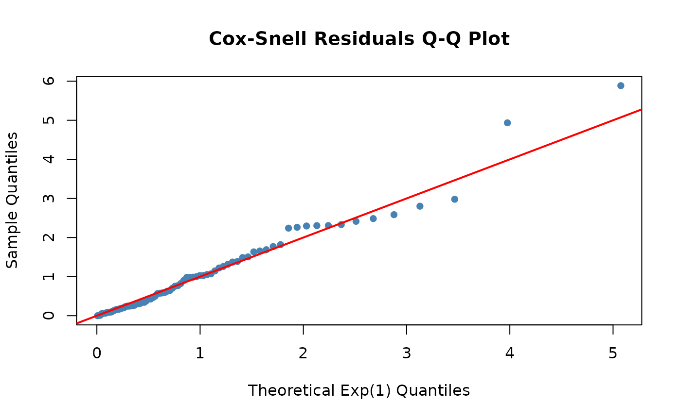

Cox-Snell residuals Q-Q plot showing model fit assessment.

Points falling along the diagonal indicate good fit. Systematic departures suggest model misspecification.

Martingale Residuals

Martingale residuals (M_i = delta_i - H(t_i)) are useful for identifying individual observations that are poorly fit:

mart_resid <- residuals(exp_final, test_df, type = "martingale")
summary(mart_resid)
#>    Min. 1st Qu.  Median    Mean 3rd Qu.    Max. 
#> -4.8856 -0.4127  0.3650  0.0000  0.7569  0.9998

# Large positive values: failed earlier than expected
# Large negative values: survived longer than expected

For more detailed diagnostic workflows, see vignette("reliability_engineering").

Summary

The flexhaz package provides:

Flexible specification: Define distributions through hazard functions
Complete distribution interface: hazard, survival, CDF, PDF, quantiles, sampling
Likelihood model support: Log-likelihood, score, Hessian for MLE
Censoring support: Handle exact and right-censored survival data
Numerical integration: Automatic computation of cumulative hazard
Model diagnostics: Residuals and Q-Q plots for fit assessment

This makes it ideal for:

Custom reliability models
Survival analysis with non-standard hazard patterns
Maximum likelihood estimation of hazard function parameters
Simulation studies with flexible failure distributions

Next Steps

vignette("getting_started") - Quick 5-minute introduction
vignette("reliability_engineering") - Five real-world case studies
vignette("custom_distributions") - The three-level optimization paradigm
vignette("custom_derivatives") - Supplying analytical score and Hessian functions