dfr.dist: Hazard-First Survival Modeling

The Problem

Standard parametric survival models force you to choose from a short list of hazard shapes: constant (exponential), monotone power-law (Weibull), exponential growth (Gompertz). But real failure patterns rarely cooperate:

• Ceramic capacitors exhibit wear-out that accelerates with age — the failure rate climbs faster than any power law.
• Software systems follow a bathtub curve: early crashes from latent bugs, a stable period, then increasing failures as dependencies rot.
• Post-surgical patients face high initial risk that drops sharply, then slowly rises again as long-term complications emerge.

Each of these demands a hazard function that standard families cannot express. You can reach for semi-parametric methods (Cox regression), but then you lose the ability to extrapolate, simulate, or compute closed-form quantities like mean time to failure.

The Idea

dfr.dist takes a different approach: you write the hazard function, and the package derives everything else.

Given a hazard (failure rate) function $h(t)$, the full distribution follows:

$$h(t) \;\xrightarrow{\;\int\;}\; H(t) = \int_0^t h(u)\,du \;\xrightarrow{\;\exp\;}\; S(t) = e^{-H(t)} \;\xrightarrow{\;\times h\;}\; f(t) = h(t)\,S(t)$$

If you can express $h(t)$ as an R function of time and parameters, dfr.dist gives you survival curves, CDFs, densities, quantiles, random sampling, log-likelihoods, MLE fitting, and residual diagnostics — automatically.

A Complete Example

Let’s model a system with a bathtub-shaped failure rate: high early risk (infant mortality), a stable useful-life period, and accelerating wear-out.

library(dfr.dist)

Define the hazard

$$h(t) = a\,e^{-bt} + c + d\,t^k$$

Three additive components: exponential decay (infant mortality), constant baseline (useful life), and power-law growth (wear-out).

bathtub <- dfr_dist(
  rate = function(t, par, ...) {
    a <- par[[1]]  # infant mortality magnitude
    b <- par[[2]]  # infant mortality decay rate
    c <- par[[3]]  # baseline hazard
    d <- par[[4]]  # wear-out coefficient
    k <- par[[5]]  # wear-out exponent
    a * exp(-b * t) + c + d * t^k
  },
  par = c(a = 0.5, b = 0.5, c = 0.01, d = 5e-5, k = 2.5)
)

Plot the hazard curve

h <- hazard(bathtub)
t_seq <- seq(0.01, 30, length.out = 300)
plot(t_seq, sapply(t_seq, h), type = "l", lwd = 2, col = "darkred",
     xlab = "Time", ylab = "Hazard rate h(t)",
     main = "Bathtub Hazard Function")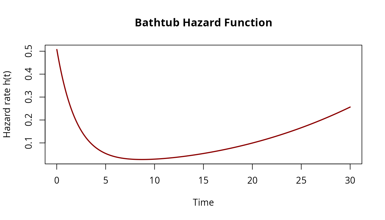

Plot the survival curve

plot(bathtub, what = "survival", xlim = c(0, 30),
     col = "darkblue", lwd = 2,
     main = "Survival Function S(t)")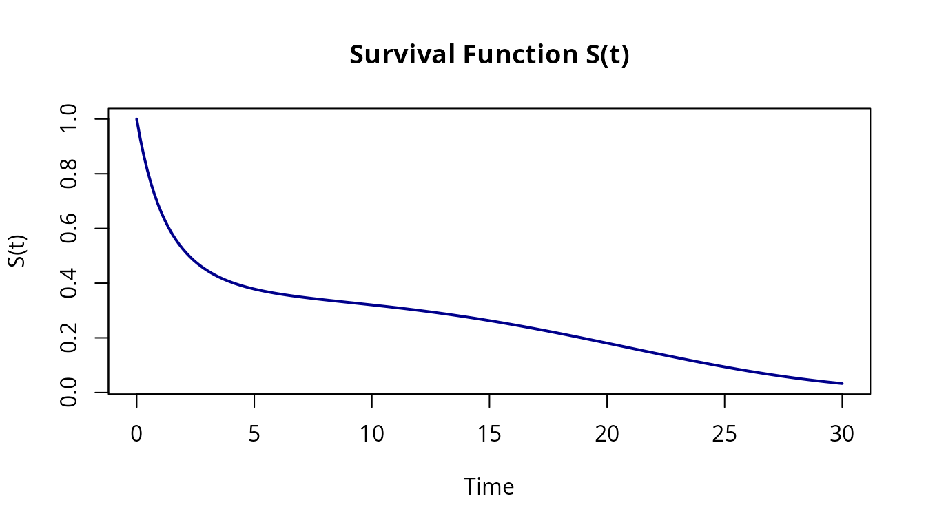

Simulate data and fit via MLE

# Generate failure times with right-censoring at t = 25
set.seed(42)
samp <- sampler(bathtub)
raw_times <- samp(80)
censor_time <- 25

df <- data.frame(
  t = pmin(raw_times, censor_time),
  delta = as.integer(raw_times <= censor_time)
)

cat("Observed failures:", sum(df$delta), "out of", nrow(df), "\n")
#> Observed failures: 68 out of 80
cat("Right-censored:", sum(1 - df$delta), "\n")
#> Right-censored: 12

# Fit the model
solver <- fit(bathtub)
result <- solver(df,
  par = c(0.3, 0.3, 0.02, 1e-4, 2),
  method = "Nelder-Mead"
)

Inspect the fit

cat("Estimated parameters:\n")
#> Estimated parameters:
print(coef(result))
#> [1] 0.4828059584 0.6478481588 0.0128496924 0.0003329348 1.7388288598

Residual diagnostics

fitted_bathtub <- dfr_dist(
  rate = function(t, par, ...) {
    par[[1]] * exp(-par[[2]] * t) + par[[3]] + par[[4]] * t^par[[5]]
  },
  par = coef(result)
)
qqplot_residuals(fitted_bathtub, df)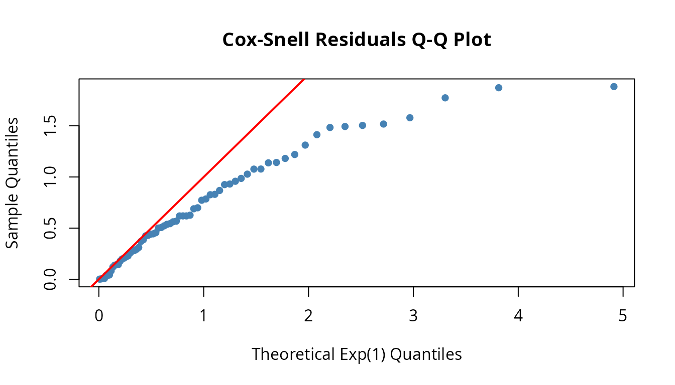

Points near the diagonal indicate the model captures the failure pattern well.

Built-in Distributions

For common parametric families, the package provides optimized constructors with analytical cumulative hazard and score functions:

Constructor	Hazard Shape	Parameters
dfr_exponential(lambda)	Constant	failure rate
dfr_weibull(shape, scale)	Power-law	shape $k$, scale $\sigma$
dfr_gompertz(a, b)	Exponential growth	initial rate, growth rate
dfr_loglogistic(alpha, beta)	Non-monotonic (hump)	scale, shape

Use these when a standard family fits your problem — they include analytical derivatives for faster, more accurate MLE.

Who Is This For?

Reliability engineers: If you think in failure rates, MTBF, and bathtub curves, dfr.dist speaks your language. Define the hazard function that matches your failure physics, fit it to test data with censoring, and extract B-life estimates, warranty predictions, and maintenance intervals — all from a single object.

Statisticians and survival analysts: If you work with censored lifetime data and need more flexibility than Weibull or Cox regression, dfr.dist gives you fully parametric models with arbitrary hazard shapes. You get proper likelihood inference (score, Hessian, confidence intervals) and residual diagnostics, with the option to supply analytical derivatives or fall back to numerical methods.

Where to Go Next

1. vignette("getting_started") — 5-minute quick start with fitting and diagnostics
2. vignette("reliability_engineering") — Five real-world case studies
3. vignette("failure_rate") — Mathematical foundations of hazard-based modeling
4. vignette("custom_distributions") — The three-level optimization paradigm
5. vignette("automatic_differentiation") — Analytical score and Hessian functions