Creating Custom Distributions • dfr.dist

The Power of Custom Hazards

The dfr.dist package lets you define any survival distribution through its hazard function (failure rate). This guide teaches you how to create your own distributions, from simple to optimized.

library(dfr.dist)

The Three Functions

Every dfr_dist can provide up to three functions:

Function	Purpose	Required?
`rate`	Hazard h(t, par)	Yes
`cum_haz_rate`	Cumulative hazard H(t, par)	Optional (computed numerically if not provided)
`score_fn`	Score function ∂ℓ/∂θ	Optional (exact gradient for faster MLE)

Let’s see how to provide each.

Level 1: Just the Hazard

The simplest approach - provide only the hazard function:

# Custom hazard: linear increasing failure rate
# h(t) = a + b*t
linear_hazard <- dfr_dist(
  rate = function(t, par, ...) {
    a <- par[[1]]
    b <- par[[2]]
    a + b * t
  },
  par = c(a = 0.1, b = 0.01)
)

# Everything else is computed automatically
h <- hazard(linear_hazard)
h(10)  # 0.1 + 0.01*10 = 0.2
#> [1] 0.2

S <- surv(linear_hazard)
S(10)  # exp(-integral of hazard)
#> [1] 0.2231302

Pros: Minimal effort, works out of the box.

Cons: Cumulative hazard computed via numerical integration (slower, less accurate).

Level 2: Add Analytical Cumulative Hazard

When you know the closed-form integral, provide it:

# H(t) = integral of (a + b*u) from 0 to t = a*t + b*t^2/2
linear_hazard_v2 <- dfr_dist(
  rate = function(t, par, ...) {
    a <- par[[1]]
    b <- par[[2]]
    a + b * t
  },
  cum_haz_rate = function(t, par, ...) {
    a <- par[[1]]
    b <- par[[2]]
    a * t + b * t^2 / 2
  },
  par = c(a = 0.1, b = 0.01)
)

# Now cumulative hazard uses the analytical formula
H <- cum_haz(linear_hazard_v2)
H(10)  # 0.1*10 + 0.01*10^2/2 = 1.5
#> [1] 1.5

# Verify survival
S <- surv(linear_hazard_v2)
S(10)  # exp(-1.5) ≈ 0.223
#> [1] 0.2231302
exp(-1.5)
#> [1] 0.2231302

Pros: Faster, exact cumulative hazard; improves all downstream computations.

Cons: More work to derive the integral.

Level 3: Add Analytical Score Function

For fastest MLE with exact Hessian, also provide the score (gradient of log-likelihood):

# Score derivation:
# Log-likelihood for exact observation: log(h(t)) - H(t)
# Log-likelihood for censored: -H(t)
#
# For exact: log(a + b*t) - a*t - b*t^2/2
# d/da: 1/(a+b*t) - t
# d/db: t/(a+b*t) - t^2/2

linear_hazard_v3 <- dfr_dist(
  rate = function(t, par, ...) {
    a <- par[[1]]
    b <- par[[2]]
    a + b * t
  },
  cum_haz_rate = function(t, par, ...) {
    a <- par[[1]]
    b <- par[[2]]
    a * t + b * t^2 / 2
  },
  score_fn = function(df, par, ...) {
    a <- par[[1]]
    b <- par[[2]]
    t <- df$t
    delta <- if ("delta" %in% names(df)) df$delta else rep(1, nrow(df))

    h_vals <- a + b * t  # hazard at each observation

    # d/da: sum over exact of 1/h(t) minus sum of all t
    da <- sum(delta / h_vals) - sum(t)

    # d/db: sum over exact of t/h(t) minus sum of all t^2/2
    db <- sum(delta * t / h_vals) - sum(t^2) / 2

    c(da, db)
  },
  par = c(a = 0.1, b = 0.01)
)

# Test: score at MLE should be near zero
set.seed(42)
test_data <- data.frame(t = sampler(linear_hazard_v3)(50), delta = 1)
solver <- fit(linear_hazard_v3)
result <- solver(test_data, par = c(0.05, 0.005))
#> Warning in log(h_exact): NaNs produced
#> Warning in log(h_exact): NaNs produced
#> Warning in log(h_exact): NaNs produced

s <- score(linear_hazard_v3)
s(test_data, par = coef(result))  # Should be ≈ (0, 0)
#> [1] -0.01503346  0.38575589

Pros: Exact gradient and Hessian; fastest optimization.

Cons: Requires deriving score function analytically.

Complete Example: Makeham Distribution

Let’s build the Makeham distribution from scratch. This models mortality with both accident (constant) and aging (exponential growth) components:

$h(t) = \lambda + \alpha e^{\beta t}$

Step 1: Derive the Mathematics

Cumulative hazard: $H(t) = \int_0^t (\lambda + \alpha e^{\beta u}) du = \lambda t + \frac{\alpha}{\beta}(e^{\beta t} - 1)$

Score function (for exact observations, delta=1): $\ell_i = \log(\lambda + \alpha e^{\beta t_i}) - \lambda t_i - \frac{\alpha}{\beta}(e^{\beta t_i} - 1)$

Derivatives: - $\frac{\partial \ell_i}{\partial \lambda} = \frac{1}{h(t_i)} - t_i$ - $\frac{\partial \ell_i}{\partial \alpha} = \frac{e^{\beta t_i}}{h(t_i)} - \frac{1}{\beta}(e^{\beta t_i} - 1)$ - $\frac{\partial \ell_i}{\partial \beta} = \frac{\alpha t_i e^{\beta t_i}}{h(t_i)} + \frac{\alpha}{\beta^2}(e^{\beta t_i} - 1) - \frac{\alpha t_i}{\beta}e^{\beta t_i}$

Step 2: Implement

dfr_makeham <- function(lambda = NULL, alpha = NULL, beta = NULL) {
  par <- if (!is.null(lambda) && !is.null(alpha) && !is.null(beta)) {
    c(lambda, alpha, beta)
  } else NULL

  dfr_dist(
    rate = function(t, par, ...) {
      lambda <- par[[1]]
      alpha <- par[[2]]
      beta <- par[[3]]
      lambda + alpha * exp(beta * t)
    },
    cum_haz_rate = function(t, par, ...) {
      lambda <- par[[1]]
      alpha <- par[[2]]
      beta <- par[[3]]
      lambda * t + (alpha / beta) * (exp(beta * t) - 1)
    },
    score_fn = function(df, par, ...) {
      lambda <- par[[1]]
      alpha <- par[[2]]
      beta <- par[[3]]
      t <- df$t
      delta <- if ("delta" %in% names(df)) df$delta else rep(1, nrow(df))

      exp_bt <- exp(beta * t)
      h_vals <- lambda + alpha * exp_bt

      # Gradient components
      dlambda <- sum(delta / h_vals) - sum(t)
      dalpha <- sum(delta * exp_bt / h_vals) - (1 / beta) * sum(exp_bt - 1)
      dbeta <- sum(delta * alpha * t * exp_bt / h_vals) +
               (alpha / beta^2) * sum(exp_bt - 1) -
               (alpha / beta) * sum(t * exp_bt)

      c(dlambda, dalpha, dbeta)
    },
    par = par
  )
}

Step 3: Test

# Create distribution
makeham <- dfr_makeham(lambda = 0.01, alpha = 0.001, beta = 0.05)

# Plot hazard
plot(makeham, what = "hazard", xlim = c(0, 50), main = "Makeham Hazard")

Makeham hazard showing constant plus exponential growth curve.


# Verify score is correct by comparing to numerical gradient
set.seed(123)
test_data <- data.frame(t = c(5, 10, 15, 20, 25), delta = c(1, 1, 0, 1, 0))

# Analytical score
s <- score(makeham)
analytical <- s(test_data, par = c(0.01, 0.001, 0.05))

# Numerical gradient
ll <- loglik(makeham)
numerical <- numDeriv::grad(function(p) ll(test_data, p), c(0.01, 0.001, 0.05))

# Should match
rbind(analytical = analytical, numerical = numerical)
#>                [,1]     [,2]     [,3]
#> analytical 178.0942 343.8909 4.836547
#> numerical  178.0942 343.8909 4.836547

Writing Custom Derivative Functions

When writing score_fn and hess_fn, follow these guidelines:

Use Standard R Indexing

# Both work fine for score_fn and hess_fn
a <- par[[1]]  # or par[1]
b <- par[[2]]  # or par[2]

Return Correct Types

# score_fn should return a numeric vector
c(da, db)

# hess_fn should return a matrix
matrix(c(d2a, d2ab, d2ab, d2b), nrow = 2)

Handle Censoring

# Always check for the delta column
delta <- if ("delta" %in% names(df)) df$delta else rep(1, nrow(df))
n_events <- sum(delta == 1)

Performance Comparison

Let’s see the speedup from analytical formulas:

# Generate test data
set.seed(42)
n <- 500
test_data <- data.frame(t = rexp(n, rate = 0.1), delta = sample(0:1, n, replace = TRUE))

# Level 1: Only hazard
dist_v1 <- dfr_dist(
  rate = function(t, par, ...) rep(par[[1]], length(t))
)

# Level 2: With cumulative hazard
dist_v2 <- dfr_dist(
  rate = function(t, par, ...) rep(par[[1]], length(t)),
  cum_haz_rate = function(t, par, ...) par[[1]] * t
)

# Level 3: With score function
dist_v3 <- dfr_exponential()  # Has all three

# Time log-likelihood evaluation
ll1 <- loglik(dist_v1)
ll2 <- loglik(dist_v2)
ll3 <- loglik(dist_v3)

# Single evaluation timing (run multiple times for accuracy)
system.time(for(i in 1:100) ll1(test_data, c(0.1)))
#>    user  system elapsed 
#>   2.154   0.020   2.175
system.time(for(i in 1:100) ll2(test_data, c(0.1)))
#>    user  system elapsed 
#>   0.383   0.000   0.383
system.time(for(i in 1:100) ll3(test_data, c(0.1)))
#>    user  system elapsed 
#>   0.367   0.000   0.367

Real-World Example: Bathtub Curve

Model the classic “bathtub” hazard with three phases:

# Bathtub: infant mortality + useful life + wear-out
# h(t) = a*exp(-b*t) + c + d*t^k
dfr_bathtub <- function(a = NULL, b = NULL, c = NULL, d = NULL, k = NULL) {
  par <- if (!is.null(a) && !is.null(b) && !is.null(c) &&
             !is.null(d) && !is.null(k)) {
    c(a, b, c, d, k)
  } else NULL

  dfr_dist(
    rate = function(t, par, ...) {
      a <- par[[1]]  # Infant mortality magnitude
      b <- par[[2]]  # Infant mortality decay
      c <- par[[3]]  # Baseline (useful life)
      d <- par[[4]]  # Wear-out coefficient
      k <- par[[5]]  # Wear-out exponent
      a * exp(-b * t) + c + d * t^k
    },
    par = par
  )
}

# Create bathtub distribution
bathtub <- dfr_bathtub(a = 0.5, b = 0.3, c = 0.02, d = 0.0001, k = 2)

# Plot the bathtub curve
plot(bathtub, what = "hazard", xlim = c(0, 20),
     main = "Bathtub Hazard Curve", col = "darkred", lwd = 2)

# Label the three phases
text(2, 0.15, "Infant\nMortality", cex = 0.8)
text(8, 0.03, "Useful Life", cex = 0.8)
text(17, 0.08, "Wear-out", cex = 0.8)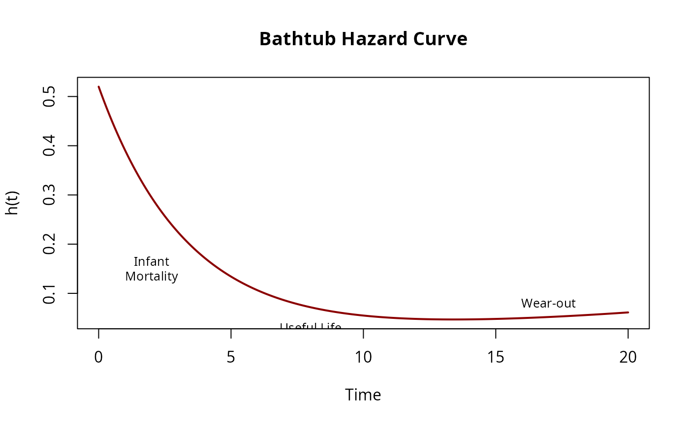

Bathtub hazard curve showing three phases: decreasing infant mortality, constant useful life, and increasing wear-out.

Summary

Level	Provide	Benefits
1	`rate` only	Quick prototyping
2	+ `cum_haz_rate`	Faster, exact survival and CDF
3	+ `score_fn`	Exact Hessian; fastest MLE

Rule of thumb:

Start with Level 1 to verify your model works
Add Level 2 if you need better performance
Add Level 3 for production-quality MLE fitting

Next Steps

vignette("reliability_engineering") - Real-world applications
vignette("automatic_differentiation") - Analytical derivatives for MLE
Package source code - Study R/distributions.R for implementation examples