Fitting Common Distributions to a DGP

library(algebraic.mle)
library(algebraic.dist)
library(boot)

Introduction

The goal of this vignette is to demonstrate using the R package algebraic.mle for inference on maximum likelihood estimators (MLEs). We will simulate a dataset whose true data generating process (DGP) is a mixture of Weibull and Normal distributions. However, we will fit Weibull and Normal distributions separately to the data to explore which provides a better fit.

Data Simulation

First, here are the simulation parameters:

n <- 100
err <- 0.1
shape <- 2
scale <- 10
theta = c(shape, scale)
set.seed(142334)

We simulate a sample of size \(n = 100\) from the DGP: \[ T_i = W_i + \epsilon_i \] where \[ W_i \sim \operatorname{Weibull}(k = 2, \lambda = 10) \] and \[ \epsilon_i \sim \operatorname{normal}(\mu = 0, \sigma = 0.1). \]

We can simulate a sample from this DGP mixture distribution using the rweibull and rnorm functions:

x <- rweibull(n = n, shape = shape, scale = scale) +
  rnorm(n = n, mean = 0, sd = err)

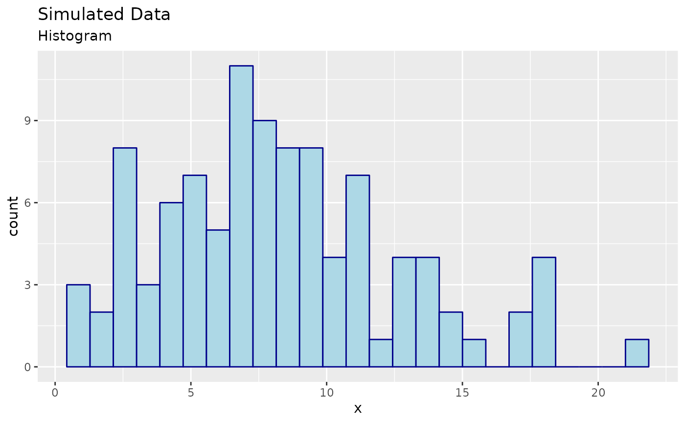
Visualizing Data

Here are some observations:

head(x, n = 4)
#> [1]  6.69  2.96 13.05  5.34

Visualizing the data is a good first step in the analysis of the data. If the data is univariate or bivariate, we can plot a histogram of the data pretty easily. We show a histogram of the simulated data below:

Parametrically Modeling the Data

If we only had this sample, what might we conclude? This can be a very difficult problem.

If we were only interested in, say, prediction, and we had a sufficiently large sample, we could use a non-parametric methods and “let the data speak for itself.” However, if we are interested in inference (e.g., explaining the data) or the sample was small, then we usually need to make some assumptions about the data.

In this case, we will assume that the data is drawn from a parametric distribution. There are many well-known, named parametric distributions, e.g., Pareto, Weibull, and Normal, to name a few. We will fit the Weibull and the Normal distributions, and compare the results.

Maximum Likelihood Estimation

We will use maximum likelihood estimation (MLE) to estimate the parameters of both the Weibull and the Normal, and then wrap these estimates into an mle object provided by algebraic.mle package:

fit_normal <- function(data) {
    loglik <- function(theta) {
        sum(dnorm(data, mean = theta[1], sd = sqrt(theta[2]), log = TRUE))
    }
    mu.hat <- mean(data)
    sigma2.hat <- mean((data - mu.hat)^2)
    H <- -numDeriv::hessian(loglik, c(mu.hat, sigma2.hat))
    mle(theta.hat = c(mu.hat, sigma2.hat),
        loglike = loglik(c(mu.hat, sigma2.hat)),
        score = numDeriv::grad(loglik, c(mu.hat, sigma2.hat)),
        sigma = MASS::ginv(H),
        info = H,
        obs = data,
        nobs = length(data),
        superclasses = c("mle_normal"))
}

fit_weibull <- function(data) {
    loglik <- function(theta) {
        sum(dweibull(data, shape = theta[1], scale = theta[2], log = TRUE))
    }

    sol <- stats::optim(
        par = c(shape, scale),
        fn = loglik,
        hessian = TRUE,
        method = "L-BFGS-B",
        lower = c(0, 0),
        #method = "Nelder-Mead",
        control = list(maxit = 10000, fnscale = -1))

    mle(theta.hat = sol$par,
        loglike = sol$value,
        sigma = MASS::ginv(-sol$hessian),
        info = -sol$hessian,
        obs = data,
        nobs = length(data),
        superclasses = c("mle_weibull"))
}

bias.mle_normal <- function(x, theta = NULL) {
    if (is.null(theta))
        theta <- params(x)
    c(0, -theta[2] / nobs(x))
}

theta.hat <- fit_normal(x)
summary(theta.hat)
#> Maximum likelihood estimator of type mle_normal is normally distributed.
#> The estimates of the parameters are given by:
#> [1]  8.23 19.11
#> The standard error is  0.437 2.7 .
#> The asymptotic 95% confidence interval of the parameters are given by:
#>         2.5% 97.5%
#> param1  7.37  9.09
#> param2 13.82 24.41
#> The MSE of the individual components in a multivariate estimator is:
#>                  [,1]             [,2]
#> [1,] 0.19112701130551 0.00000000000607
#> [2,] 0.00000000000607 7.34243642454061
#> The log-likelihood is  -289 .
#> The AIC is  583 .

theta.weibull <- fit_weibull(x)
summary(theta.weibull)
#> Maximum likelihood estimator of type mle_weibull is normally distributed.
#> The estimates of the parameters are given by:
#> [1] 1.95 9.27
#> The standard error is  0.153 0.5 .
#> The asymptotic 95% confidence interval of the parameters are given by:
#>        2.5% 97.5%
#> param1 1.65  2.25
#> param2 8.29 10.25
#> The MSE of the individual components in a multivariate estimator is:
#>        [,1]   [,2]
#> [1,] 0.0235 0.0237
#> [2,] 0.0237 0.2497
#> The log-likelihood is  -284 .
#> The AIC is  573 .

Let’s plot the pdfs of the Weibull and normal distributions:

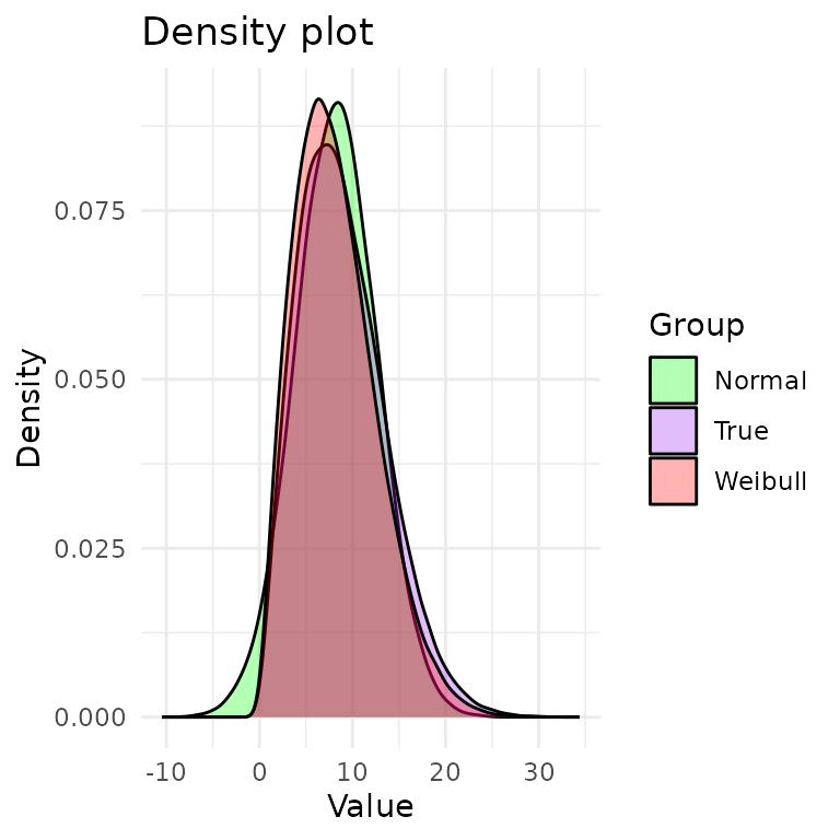
In purple, we have the true density (DGP). In red, we have the Weibull density. In green, we have the normal density. From the plot, it’s hard to tell which distribution is a better fit to the DGP.

Interestingly, the tails of the true distribution seem a bit heavier than the tails of the Weibull and Normal. This may suggest that a heavier-tailed model may be a better fit, such as the lognormal distribution, but we will not pursue this.

Performance Measures of the MLE

A nice property of MLEs is that, asymptotically, given some regularity conditions, they are normally distributed with a mean given by the true true parameter and a variance-covariance given by the inverse of the FIM evaluated at \(\theta\).

We do not know \(\theta\), but we have have estimates, and thus we may approximate the sampling distribution of \(\hat\theta\) with \(\mathcal{N}(\hat\theta,I^{-1}(\hat\theta))\).

Let \(F\) denote the true distribution function such that \(X_j \sim F\) for all \(j\). Suppose we have some population parameter \(\theta = t(F)\) and an estimator of \(\theta\) given by \(\hat\theta = s(\{X_1,\ldots,X_n\})\). A reasonable requirement for an estimator \(\hat\theta\) is that it converges to the true parameter value \(\theta\) as we collect more and more data. In particular, we say that it is a consistent estimator of \(\theta\) if \(\hat\theta\) converges in probability to \(\theta\), denoted by \(\hat\theta \overset{p}{\mapsto} \theta\).

If the regularity conditions hold for the MLE, then \(\hat\theta\) is a consistent estimator of \(\theta\). However, for finite sample sizes, the estimator may be biased. The bias of \(\hat\theta\) with respect to \(\theta\) is defined as \[ \operatorname{bias}(\hat\theta,\theta) = E(\hat\theta) - \theta, \] where \(\operatorname{bias}(\hat\theta,\theta) = 0\) indicates that \(\hat\theta\) is an unbiased estimator of \(\theta\).

As a function of the true distribution \(F\), the bias is unknown and is not a statistic. However, in the case of the normal, \(\hat\mu\) is unbiased and, analytically, the bias of \(\hat\sigma^2\) is given by \(-\frac{1}{n} \sigma^2\):

bias(theta.hat,theta)
#> [1]  0.0 -0.1

If \(\sigma^2\) is not known, we may estimate it by using replacing \(\hat\sigma^2\) instead:

bias(theta.hat)
#> [1]  0.000 -0.191

This is pretty far off from the true bias. This may be the first indication that the DGP is far from being normal.

If we wanted to estimate the bias for the Weibull, we could bootstrap it or something else, but we don’t attempt to do that here.

The mean squared error (MSE) is another performance measure of an estimator. It is given by \[ \operatorname{mse}(\hat\theta) = E\bigl\{(\hat\theta - \theta)^T(\hat\theta - \theta)\bigr\}, \] Another way to compute the MSE is given by \[ \operatorname{mse}(\hat\theta) = \operatorname{trace}(\operatorname{cov}(\hat\theta) + \operatorname{bias}(\hat\theta)^T \operatorname{bias}(\hat\theta). \]

Here’s R code to compute the MSE of \(\hat\theta\):

round(mse(theta.hat), digits=3)
#>       [,1] [,2]
#> [1,] 0.191 0.00
#> [2,] 0.000 7.34
round(mse(theta.weibull), digits=3)  # true MSE
#>       [,1]  [,2]
#> [1,] 0.023 0.024
#> [2,] 0.024 0.250

The normal distribution has significant MSE compared to the Weibull.

Invariance Property of the MLE

An interesting property of an MLE \(\hat\theta\) is that the MLE of \(f(\theta)\) is given by \(f(\hat\theta)\). What is the distribution of \(f(\hat\theta)\)? Asymptotically, it is normally distributed with a mean given by \(f(\theta)\) and a variace-covariance given by the covariance of the sampling distribution of \(f(\hat\theta)\).

We provide two methods to compute the variance-covariance.

Delta Method

If \(f\) is differentiable, the variance-covariance is given by \[ \operatorname{var}(f(\hat\theta)) = \operatorname{E}\bigl\{ \bigl(f(\hat\theta) - f(\theta)\bigr)^2\bigr\} = \operatorname{E}\bigl\{J_f(\hat\theta) I(\hat\theta)^{-1} J_f(\hat\theta)^T\bigr\}. \] Here, \(J_f(\hat\theta)\) is the Jacobian of \(f\) evaluated at \(\hat\theta\).

Monte-Carlo Method

The delta method requires that \(f\) be differentiable, but we may use the Monte-carlo method to estimate the distribution of \(f(\hat\theta)\) for any function \(f\). We simply sample from the MLE of \(\hat\theta\) and apply \(f\) to its estimates and take the covariance of the sample.

Next, we show how to compute the sampling distribution of \(g(\hat\theta)\) for some function \(g\) and some MLE \(\hat\theta\) using both the delta and mc methods.

Example 1

For this example, we use the Weibull fit. Let \(g(\theta) = A \theta + b\) for some matrix \(A\) and vector \(b\). (This is a simple linear transformation of \(\theta\).) We can define \(g\) in R with:

A <- matrix(c(2,3),nrow=2)
b <- c(1,0)
g <- function(x) A %*% x + b

We compute the variance-covariance of the MLE of \(g(\theta)\) using both methods:

g.mc <- rmap(theta.weibull,g,n=100000L)
g.delta <- rmap(theta.weibull,g,method="delta")
round(vcov(g.mc), digits=3)
#>       [,1]  [,2]  [,3]  [,4]
#> [1,] 0.095 0.142 0.095 0.143
#> [2,] 0.142 0.213 0.143 0.214
#> [3,] 0.095 0.143 1.003 1.504
#> [4,] 0.143 0.214 1.504 2.256
round(vcov(g.delta), digits=3)
#>       [,1]  [,2]  [,3]  [,4]
#> [1,] 0.094 0.141 0.095 0.142
#> [2,] 0.141 0.211 0.142 0.213
#> [3,] 0.095 0.142 0.999 1.498
#> [4,] 0.142 0.213 1.498 2.247

They are pretty close.

Weighted MLE: A Weighted Sum of MLEs

Since the variance-covariance of an MLE is inversely proportional to the Fisher information that the MLE is defined with respect to, we can combine multiple MLEs of \(\theta\), each of which may be defined with respect to a different kind of sample, to arrive at the MLE that incorporates the Fisher information in all of those samples.

Consider \(k\) mutually independent MLEs of parameter \(\theta\), \(\hat\theta_1,\ldots,\hat\theta_k\), where \(\hat\theta_j \sim N(\theta,I_j^{-1}(\theta))\). Then, the sampling MLE of \(\theta\) that incorporates all of the data in \(\hat\theta_1,\ldots,\hat\theta_k\) is given by the inverse-variance weighted mean, \[ \hat\theta_w = \left(\sum_{j=1}^k I_j(\theta)\right)^{-1} \left(\sum_{j=1}^k I_j(\theta) \hat\theta_j\right), \] which, asymptotically, has an expected value of \(\theta\) and a variance-covariance of \(\left(\sum_{j=1}^k I_j(\theta)\right)^{-1}\).

Example 2

For this example, we use the normal fit.

To evaluate the performance of the weighted MLE, we generate a sample of \(N=1000\) observations from \(\mathcal{N}(\theta)\) and compute the MLE for the observed sample, denoted by \(\hat\theta\).

We then divide the observed sample into \(r=5\) sub-samples, each of size \(N/r=100\), and compute the MLE for each sub-sampled, denoted by \(\theta^{(1)},\ldots,\theta^{(r)}\).

Finally, we do a weighted combination these MLEs to form the weighted MLE, denoted by \(\theta_w\):

N <- 500
r <- 5
samp <- rnorm(N, mean = theta[1], sd = sqrt(theta[2]))
samp.sub <- matrix(samp, nrow = r)
mles.sub <- list(length = r)
for (i in 1:r)
    mles.sub[[i]] <- fit_normal(samp.sub[i,])

mle.wt <- mle_weighted(mles.sub)
mle <- fit_normal(samp)

We show the results in the following R code. First, we show the weighted MLE and its MSE:

params(mle.wt)
#> [1] 1.98 8.71
round(mse(mle.wt), digits=3)
#>       [,1]  [,2]
#> [1,] 0.018 0.000
#> [2,] 0.000 0.313

The MLE for the total sample and its MSE is:

params(mle)
#> [1] 1.98 9.28
round(mse(mle), digits=3)
#>       [,1]  [,2]
#> [1,] 0.019 0.000
#> [2,] 0.000 0.345

We see that \(\hat\theta\) and \(\hat\theta_w\) model approximately the same sampling distribution.

Bootstrapping the MLEs

Let’s compare the earlier results that relied on the large sampling assumption with the bootstrapped MLE using mle_boot. First, mle_boot is just a wrapper for boot objects or objects like boot. Thus to use mle_boot, we first need to call boot to bootstrap our MLE for the Weibull fit.

We just need to wrap it in a function that takes the data as input and returns the MLE of the parameters and then pass it to mle_boot constructor:

theta.boot <- mle_boot(
    boot(data = x,
         statistic = function(x, i) params(fit_weibull(x[i])),
         R = 1000))

We already printed out the theta.boot object, which provided a lot of information about it, but we can obtain specified statistics from the Bootstrap MLE using the standard interface in algorithmic.mle, e.g.:

print(theta.boot)
#> Maximum likelihood estimator of type mle_boot is normally distributed.
#> The estimates of the parameters are given by:
#> [1] 1.95 9.27
#> The standard error is  0.153 0.501 .
#> The asymptotic 95% confidence interval of the parameters are given by:
#>        2.5% 97.5%
#> param1 1.64  2.23
#> param2 8.31 10.28
#> The MSE of the individual components in a multivariate estimator is:
#>        [,1]   [,2]
#> [1,] 0.0235 0.0283
#> [2,] 0.0283 0.2519
bias(theta.boot)
#> [1]  0.0159 -0.0228

We see that, for the most part, the results are similar to those obtained using the large sampling assumption.

Goodness-of-Fit

We are fitting a model to the data that does not precisely capture the generative model \(W\). So, how good of a fit is it?

We will conduct a goodness of fit test, \[\begin{align} H_0 &: \text{the data is compatible with the Weibull distribution}\\ H_A &: \text{the data is not compatible with the Weibull distribution}. \end{align}\]

To perform this test, we will use the Cramer-von Mises test. This test is based on the Cramer-von Mises statistic, which is a measure of the distance between the empirical distribution function of the data and the distribution function of the model. The Cramer-von Mises statistic is given by \[ \hat D_n^2 = \frac{1}{n}\sum_{i=1}^n \left(\hat F_n(x_i) - F(x_i)\right)^2 \] where \(\hat F_n\) is the empirical distribution function of the data and \(F\) is the distribution function of the model.

cramer.test <- function(obs.dat,ref.dat)
{
  stat <- CDFt::CramerVonMisesTwoSamples(obs.dat,ref.dat)
  list(p.value=exp(-stat)/6.0,
       cramer.stat=stat,
       obs.size=length(obs.dat),
       ref.size=length(ref.dat))
}

wei.shape <- params(theta.weibull)[1]
wei.scale <- params(theta.weibull)[2]
ref.dat <- rweibull(1000000, shape = wei.shape, scale = wei.scale)
cramer.test(x, ref.dat)
#> $p.value
#> [1] 0.16
#> 
#> $cramer.stat
#> [1] 0.042
#> 
#> $obs.size
#> [1] 100
#> 
#> $ref.size
#> [1] 1000000

Looking at the \(p\)-value, we see that the data is compatible with the Weibull distribution. Now, let’s do the same for the normal distribution:

norm.mu <- params(theta.hat)[1]
norm.var <- params(theta.hat)[2]
ref.dat <- rnorm(1000000, mean = norm.mu, sd = sqrt(norm.var))
cramer.test(x, ref.dat)
#> $p.value
#> [1] 0.149
#> 
#> $cramer.stat
#> [1] 0.112
#> 
#> $obs.size
#> [1] 100
#> 
#> $ref.size
#> [1] 1000000

They are both compatible with the data. However, the Weibull distribution has a larger \(p\)-value, which may suggest it is a better fit. We also have the AIC measure of goodness of fit. The AIC is given by \[ \text{AIC} = -2\log L + 2k, \] where \(L\) is the likelihood of the model and \(k\) is the number of parameters in the model. The AIC is a measure of the tradeoff between the goodness of fit and the complexity of the model.

aic(theta.weibull)
#> [1] 573
aic(theta.hat)
#> [1] 583

A lower AIC value indicates a better fit. Thus, according to this measure, the Weibull distribution is the better fit.

Prediction Intervals

Frequently, we are actually interested in predicting the outcome of the random variable (or vector) that we are estimating the parameters of.

We observed a sample \(\mathcal{D} = \{T_i\}_{i=1}^n\) where \(T_i \sim N(\mu,\sigma^2)\), \(\theta = (\mu,\sigma^2)^T\) is not known. We compute the MLE of \(\theta\), which, asymptotically, is normally distributed with a mean \(\theta\) and a variance-covariance \(I^{-1}(\theta)/n\).

We wish to model the uncertainty of a new observation, \(\hat{T}_{n+1}|\mathcal{D}\). We do so by considering both the uncertainty inherent to the Normal distribution and the uncertainty of our estimate \(\hat\theta\) of \(\theta\). In particular, we let \(\hat{T}_{n+1}|\hat\theta \sim N(\hat\mu,\hat\sigma^2)\) and \(\hat\theta \sim N(\theta,I^{-1}(\theta)/n)\) (the sampling distribution of the MLE). Then, the joint distribution of \(\hat{T}_{n+1}\) and \(\hat\theta\) has the pdf given by \[ f(t,\theta) = f_{\hat{T}|\hat\theta}(t|\theta=(\mu,\sigma^2)) f_{\hat\theta}(\theta), \] and thus to find \(f(t)\), we marginalize over \(\theta\), obtaining \[ f(t) = \int_{-\infty}^\infty \int_{-\infty}^{\infty} f_{\hat{T}_{n+1},\hat\mu,\hat\sigma^2}(t,\mu,\sigma^2) d\mu d\sigma^2. \]

Given the information in the sample, the uncertainty in the new observation is characterized by the distribution \[ \hat{T}_{n+1} \sim f(t). \]

It has greater variance than \(T_{n+1}|\hat\theta\) because, as stated earlier, we do not know \(\theta\), we only have an uncertain estimate \(\hat\theta\).

In pred, we compute the predictive interval (PI) of the distribution of \(\hat{T}_{n+1}\) using Monte Carlo simulation, where we replace the integral with a sum over a large number of draws from the joint distribution of \(\hat{T}_{n+1}\) and \(\hat\theta\) and then compute the empirical quantiles.

The function pred takes as arguments x, in this case an mle object, and a sampler for the distribution of the random variable of interest, in this case rweibull (the sampler for the normal distribution). The sampler must be compatible with the output of point(x), whether that output be a scalar or a vector. Here is how we compute the PI for \(\hat{T}_{n+1}\):

pred(x=theta.hat, samp=function(n=1, theta) rnorm(n,theta[1],theta[2]))
#>      mean lower upper
#> [1,] 8.39 -29.8  46.6

In general, it will return a \(p\)-by-\(3\) matrix, where \(p\) is the dimension of \(T\) and the columns are the mean, lower quantile, and upper quantile of the predictive distribution.

How does this compare to \(T_{n+1}|\hat\theta\)? We can compute the 95% quantile interval for \(T_{n+1}|\hat\theta\) using the qnorm function:

mu <- params(theta.hat)[1]
sd <- sqrt(params(theta.hat)[2])
c(mean=mu,lower=qnorm(.025,mean=mu, sd=sd),upper=qnorm(.975,mean=mu, sd=sd))
#>   mean  lower  upper 
#>  8.230 -0.338 16.799

We see that the 95% quantile interval for \(T_{n+1}|\hat\theta\) is smaller than \(\hat{T}_{n+1}\), which is what we expected. After all, there is uncertainty about the parameter value \(\theta\).

Conclusion

In this vignette, we demonstrated how to use the algebraic.mle package to estimate the sampling distribution of the MLE using the large sampling assumption and the Bootstrap method. The package provides various functions for obtaining statistics of the MLE, allowing for a deeper understanding of the properties of your estimator.

We showed how to fit Weibull and Normal distributions to a simulated dataset whose true distribution, while known, does not have a common name.

We have shown how to compare the two models using the Cramer-von Mises test and the AIC measure of goodness of fit. We came to no definitive conclusion about which model is better, but the Weibull distribution has a larger \(p\)-value from the Cramer-von Mises test, and a lower AIC value, which serves as some evidence that it is a better fit. We saw the true DGP is visually different from both the Weibull and the normal distributions. Notably, the DGP has longer tails than both, suggesting that an even better fit may be a long-tail distribution like the log-normal or the Pareto distribution.