Likelihood Named Distributions Model
Source:vignettes/likelihood-name-model.Rmd
likelihood-name-model.RmdIntroduction
The likelihood_name() function creates a likelihood
model for any standard R distribution by name. If R has functions
d<name> (PDF) and p<name> (CDF)
for a distribution, you can build a likelihood model for it with a
single call.
This approach is ideal when:
- You want to quickly fit a standard distribution to data
- Your data may include exact, left-censored, right-censored, or interval-censored observations
- You don’t need hand-derived analytical derivatives (numerical differentiation is used by default)
For performance-critical applications with known analytical
derivatives, see the specialized models
(weibull_uncensored, exponential_lifetime) or
the likelihood_contr_model for custom likelihood
contributions.
Tip: These models can also serve as building blocks inside a
likelihood_contr_modelfor heterogeneous observation types.
Basic Usage: Normal Distribution
The simplest case: all observations are exact (no censoring).
# Generate data from N(5, 2)
set.seed(42)
n <- 200
df <- data.frame(x = rnorm(n, mean = 5, sd = 2))

# Create model -- no censor_col means all exact
model <- likelihood_name("norm", ob_col = "x")
print(model)
#> Likelihood model: likelihood_name_norm
#> ---------------
#> Observation column: x
#> Assumptions:
#>  - independent observations
#>  - identically distributed
#>  - norm distribution

# Fit the MLE
mle <- fit(model)(df, par = c(mean = 0, sd = 1))
summary(mle)
#> Maximum Likelihood Estimate (Fisherian)
#> ----------------------------------------
#>
#> Coefficients:
#>      Estimate Std. Error    2.5% 97.5%
#> mean  4.94435    0.13750 4.67485 5.214
#> sd    1.94459    0.09725 1.75398 2.135
#>
#> Log-likelihood: -416.8
#> AIC: 837.5
#> Number of observations: 200
The fisher_mle object provides standard inference:
Right-Censored Data
Right-censoring is common in survival analysis: we know the event hadn’t occurred by the censoring time, but not when it actually occurs. The likelihood contribution for a right-censored observation at is .
# Simulate Weibull lifetimes with type-I right-censoring at time 1.2
set.seed(123)
n <- 150
true_shape <- 2
true_scale <- 1.5
censor_time <- 1.2

raw_t <- rweibull(n, true_shape, true_scale)
df_right <- data.frame(
  x = pmin(raw_t, censor_time),
  censor = ifelse(raw_t > censor_time, "right", "exact")
)

cat("Censoring rate:", mean(df_right$censor == "right") * 100, "%\n")
#> Censoring rate: 53.33 %

# Fit with proper censoring handling
model_right <- likelihood_name("weibull", ob_col = "x", censor_col = "censor")
mle_right <- fit(model_right)(df_right, par = c(shape = 1.5, scale = 1))

cat("\nMLE (with censoring):\n")
#>
#> MLE (with censoring):
cat("  shape:", coef(mle_right)[1], "(true:", true_shape, ")\n")
#>   shape: 1.953 (true: 2 )
cat("  scale:", coef(mle_right)[2], "(true:", true_scale, ")\n")
#>   scale: 1.517 (true: 1.5 )
confint(mle_right)
#>        2.5% 97.5%
#> shape 1.527 2.378
#> scale 1.306 1.727
Left-Censored Data
Left-censoring occurs when observations fall below a detection limit. For example, a chemical assay might report “below 0.1 ppm” rather than an exact concentration. The likelihood contribution is .
# Simulate concentrations from a log-normal distribution
# with detection limit at 0.5
set.seed(456)
n <- 100
true_meanlog <- 0
true_sdlog <- 0.8
detect_limit <- 0.5

raw_conc <- rlnorm(n, true_meanlog, true_sdlog)
df_left <- data.frame(
  x = ifelse(raw_conc < detect_limit, detect_limit, raw_conc),
  censor = ifelse(raw_conc < detect_limit, "left", "exact")
)

cat("Below detection limit:", mean(df_left$censor == "left") * 100, "%\n")
#> Below detection limit: 16 %

model_left <- likelihood_name("lnorm", ob_col = "x", censor_col = "censor")
mle_left <- fit(model_left)(df_left, par = c(meanlog = 0, sdlog = 1))

cat("\nMLE (accounting for detection limit):\n")
#>
#> MLE (accounting for detection limit):
cat("  meanlog:", coef(mle_left)[1], "(true:", true_meanlog, ")\n")
#>   meanlog: 0.09801 (true: 0 )
cat("  sdlog:  ", coef(mle_left)[2], "(true:", true_sdlog, ")\n")
#>   sdlog:   0.7992 (true: 0.8 )
Interval-Censored Data
Interval censoring arises when we only know an observation falls within a range . This is common with grouped data, periodic inspections, or binned measurements.
The likelihood contribution is .
To use interval censoring, specify ob_col_upper for the
upper-bound column:
# Simulate inspection data: items are checked at fixed intervals
# and we only know failure occurred between two inspection times
set.seed(789)
n <- 120
true_shape <- 3
true_scale <- 5

raw_t <- rweibull(n, true_shape, true_scale)
# Inspection every 1 unit of time
inspection_lower <- floor(raw_t)
inspection_upper <- ceiling(raw_t)
# Ensure lower < upper
inspection_upper <- ifelse(inspection_lower == inspection_upper,
                           inspection_upper + 1, inspection_upper)

df_interval <- data.frame(
  x = inspection_lower,
  x_upper = inspection_upper,
  censor = rep("interval", n)
)

head(df_interval)
#>   x x_upper   censor
#> 1 3       4 interval
#> 2 6       7 interval
#> 3 8       9 interval
#> 4 4       5 interval
#> 5 4       5 interval
#> 6 7       8 interval

model_interval <- likelihood_name("weibull", ob_col = "x",
                                  censor_col = "censor",
                                  ob_col_upper = "x_upper")
mle_interval <- fit(model_interval)(df_interval, par = c(shape = 2, scale = 4))

cat("MLE from interval-censored data:\n")
#> MLE from interval-censored data:
cat("  shape:", coef(mle_interval)[1], "(true:", true_shape, ")\n")
#>   shape: 3.354 (true: 3 )
cat("  scale:", coef(mle_interval)[2], "(true:", true_scale, ")\n")
#>   scale: 5.163 (true: 5 )
Mixed Censoring Types
Real datasets often combine multiple censoring mechanisms. The model handles all four types simultaneously:
set.seed(101)
n <- 200
true_mean <- 10
true_sd <- 3

raw_x <- rnorm(n, true_mean, true_sd)

# Simulate mixed censoring:
# - 60% exact observations
# - 15% right-censored (above upper limit)
# - 15% left-censored (below detection limit)
# - 10% interval-censored (binned to nearest integer)
detect_lower <- 5
detect_upper <- 14

censor_type <- character(n)
x_obs <- numeric(n)
x_upper <- rep(NA_real_, n)

for (i in seq_len(n)) {
  if (raw_x[i] < detect_lower) {
    censor_type[i] <- "left"
    x_obs[i] <- detect_lower
  } else if (raw_x[i] > detect_upper) {
    censor_type[i] <- "right"
    x_obs[i] <- detect_upper
  } else if (runif(1) < 0.15) {
    # Some exact observations get binned
    censor_type[i] <- "interval"
    x_obs[i] <- floor(raw_x[i])
    x_upper[i] <- ceiling(raw_x[i])
    if (x_obs[i] == x_upper[i]) x_upper[i] <- x_upper[i] + 1
  } else {
    censor_type[i] <- "exact"
    x_obs[i] <- raw_x[i]
  }
}

df_mixed <- data.frame(x = x_obs, x_upper = x_upper, censor = censor_type)
cat("Censoring breakdown:\n")
#> Censoring breakdown:
print(table(df_mixed$censor))
#>
#>    exact interval     left    right
#>      147       24       11       18

model_mixed <- likelihood_name("norm", ob_col = "x", censor_col = "censor",
                               ob_col_upper = "x_upper")
mle_mixed <- fit(model_mixed)(df_mixed, par = c(mean = 8, sd = 2))

cat("\nMLE with mixed censoring:\n")
#>
#> MLE with mixed censoring:
cat("  mean:", coef(mle_mixed)[1], "(true:", true_mean, ")\n")
#>   mean: 9.908 (true: 10 )
cat("  sd:  ", coef(mle_mixed)[2], "(true:", true_sd, ")\n")
#>   sd:   2.984 (true: 3 )
confint(mle_mixed)
#>       2.5%  97.5%
#> mean 9.490 10.327
#> sd   2.653  3.314
Multiple Distributions
The likelihood_name() function works with any
distribution that follows R’s naming convention
(d<name>, p<name>). Here are a few
examples:
set.seed(202)

# Exponential
df_exp <- data.frame(x = rexp(200, rate = 2.5))
mle_exp <- fit(likelihood_name("exp", "x"))(df_exp, par = c(rate = 1))
cat("Exponential: rate =", coef(mle_exp), "(true: 2.5)\n")
#> Exponential: rate = 2.345 (true: 2.5)

# Gamma
df_gam <- data.frame(x = rgamma(200, shape = 3, rate = 2))
mle_gam <- fit(likelihood_name("gamma", "x"))(df_gam, par = c(shape = 1, rate = 1))
cat("Gamma: shape =", coef(mle_gam)[1], "rate =", coef(mle_gam)[2],
    "(true: 3, 2)\n")
#> Gamma: shape = 2.738 rate = 1.757 (true: 3, 2)

# Log-normal
df_lnorm <- data.frame(x = rlnorm(200, meanlog = 1, sdlog = 0.5))
mle_lnorm <- fit(likelihood_name("lnorm", "x"))(df_lnorm,
                                                  par = c(meanlog = 0, sdlog = 1))
cat("Log-normal: meanlog =", coef(mle_lnorm)[1], "sdlog =", coef(mle_lnorm)[2],
    "(true: 1, 0.5)\n")
#> Log-normal: meanlog = 0.9719 sdlog = 0.5154 (true: 1, 0.5)
Fisherian Inference
The likelihood.model package supports pure
likelihood-based inference in the Fisherian tradition. After fitting a
model, we can examine the likelihood surface directly without making
probability statements about parameters.
# Fit a normal model
set.seed(303)
df <- data.frame(x = rnorm(150, mean = 5, sd = 2))
model <- likelihood_name("norm", ob_col = "x")
mle <- fit(model)(df, par = c(0, 1))

# Support function: S(theta) = logL(theta) - logL(theta_hat)
# At the MLE, support is always 0
s_mle <- support(mle, coef(mle), df, model)
cat("Support at MLE:", s_mle, "\n")
#> Support at MLE: 0

# At other values, support is negative
s_alt <- support(mle, c(4, 3), df, model)
cat("Support at (4, 3):", s_alt, "\n")
#> Support at (4, 3): -30.75

# Relative likelihood: R(theta) = L(theta)/L(theta_hat) = exp(S(theta))
rl <- relative_likelihood(mle, c(4, 3), df, model)
cat("Relative likelihood at (4, 3):", rl, "\n")
#> Relative likelihood at (4, 3): 4.42e-14
Likelihood Intervals
A likelihood interval contains all parameter values whose relative likelihood exceeds . The interval is roughly analogous to a 95% confidence interval but makes no probability statement about the parameter.
# 1/8 likelihood interval for the mean (parameter 1)
li <- likelihood_interval(mle, df, model, k = 8, param = 1)
cat("1/8 likelihood interval for mean:\n")
#> 1/8 likelihood interval for mean:
print(li)
#> 1/8 Likelihood Interval (R >= 0.125)
#> -----------------------------------
#>      lower upper
#> [1,] 4.748 5.403
#> attr(,"k")
#> [1] 8
#> attr(,"relative_likelihood_cutoff")
#> [1] 0.125

# Compare with Wald CI
cat("\nWald 95% CI:\n")
#>
#> Wald 95% CI:
print(confint(mle))
#>       2.5% 97.5%
#> [1,] 4.763 5.388
#> [2,] 1.733 2.176
Profile Likelihood
The profile likelihood for a single parameter maximizes over all other parameters at each fixed value, giving a one-dimensional view of the likelihood surface.
prof <- profile_loglik(mle, df, model, param = 1, n_grid = 30)

plot(prof[[1]], prof$relative_likelihood, type = "l",
     xlab = "Mean", ylab = "Relative likelihood",
     main = "Profile likelihood for mean parameter")
abline(h = 1/8, lty = 2, col = "gray")
abline(v = coef(mle)[1], lty = 2, col = "blue")
legend("topright", legend = c("Profile R(mean)", "1/8 cutoff", "MLE"),
       lty = c(1, 2, 2), col = c("black", "gray", "blue"), cex = 0.8)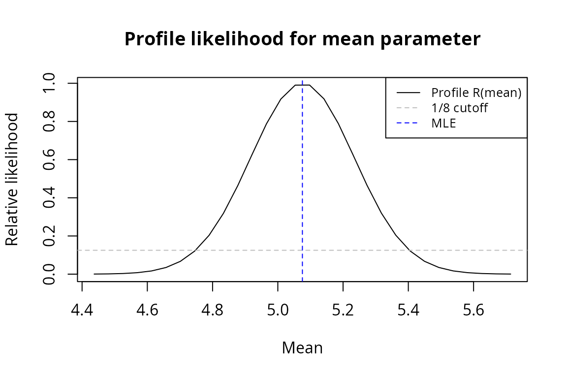
Comparison with Specialized Models
The generic likelihood_name("exp", ...) produces the
same log-likelihood as the specialized
exponential_lifetime(), but the latter provides analytical
derivatives and a closed-form MLE:
set.seed(404)
x <- rexp(150, rate = 2.0)

# Generic approach
df_gen <- data.frame(t = x, censor = rep("exact", length(x)))
model_gen <- likelihood_name("exp", ob_col = "t", censor_col = "censor")
ll_gen <- loglik(model_gen)(df_gen, 2.0)

# Specialized approach
df_spec <- data.frame(t = x)
model_spec <- exponential_lifetime("t")
ll_spec <- loglik(model_spec)(df_spec, 2.0)

cat("Generic loglik:     ", ll_gen, "\n")
#> Generic loglik:      -31
cat("Specialized loglik: ", ll_spec, "\n")
#> Specialized loglik:  -31
cat("Match:", all.equal(ll_gen, ll_spec), "\n")
#> Match: TRUE
The specialized model is faster because it bypasses
do.call overhead and provides analytical score and
Hessian:
# Generic: uses optim
mle_gen <- fit(model_gen)(df_gen, par = c(rate = 1))

# Specialized: closed-form MLE, no optimization needed
mle_spec <- fit(model_spec)(df_spec)

cat("Generic MLE:     ", coef(mle_gen), "\n")
#> Generic MLE:      2.223
cat("Specialized MLE: ", coef(mle_spec), "\n")
#> Specialized MLE:  2.223
Parameter Naming Conventions
The prepare_args_list() function (used internally)
matches your parameter vector to the distribution function’s formals.
You can pass named or unnamed parameters:
model <- likelihood_name("norm", ob_col = "x")
ll <- loglik(model)
df <- data.frame(x = rnorm(50, 5, 2))

# Both produce identical results:
ll_named <- ll(df, c(mean = 5, sd = 2))
ll_unnamed <- ll(df, c(5, 2))
cat("Named:", ll_named, "\n")
#> Named: -104.9
cat("Unnamed:", ll_unnamed, "\n")
#> Unnamed: -104.9
cat("Match:", ll_named == ll_unnamed, "\n")
#> Match: TRUE
For distributions with many parameters, naming helps avoid mistakes.
The function matches by position for unnamed parameters, using the
distribution’s formal arguments (excluding x,
log, lower.tail, etc.):
# Gamma has formals: shape, rate (or scale)
# dnorm has formals: mean, sd
cat("dnorm formals:", paste(names(formals(dnorm)), collapse = ", "), "\n")
#> dnorm formals: x, mean, sd, log
cat("dgamma formals:", paste(names(formals(dgamma)), collapse = ", "), "\n")
#> dgamma formals: x, shape, rate, scale, log
cat("dweibull formals:", paste(names(formals(dweibull)), collapse = ", "), "\n")
#> dweibull formals: x, shape, scale, log
Passing too many parameters produces a clear error:
ll(df, c(0, 1, 0.5))  # 3 params for 2-param distribution
#> Error in prepare_args_list(par, model$pdf): Too many parameters (3) for distribution (expects at most 2: mean, sd)
Hypothesis Testing
The likelihood ratio test compares nested models. Here we test whether an exponential distribution fits data that was actually generated from a Weibull:
set.seed(505)
df_test <- data.frame(x = rweibull(200, shape = 1.8, scale = 2))

# Fit both models
model_exp <- likelihood_name("exp", ob_col = "x")
model_weib <- likelihood_name("weibull", ob_col = "x")

mle_exp_test <- fit(model_exp)(df_test, par = c(rate = 0.5))
mle_weib_test <- fit(model_weib)(df_test, par = c(shape = 1, scale = 1))

cat("Exponential loglik:", loglik_val(mle_exp_test), "\n")
#> Exponential loglik: -318.7
cat("Weibull loglik:    ", loglik_val(mle_weib_test), "\n")
#> Weibull loglik:     -275.8

# LRT: exponential (1 param) vs Weibull (2 params)
lrt_result <- lrt(model_exp, model_weib, df_test,
                  null_par = coef(mle_exp_test),
                  alt_par = coef(mle_weib_test),
                  dof = 1)
print(lrt_result)
#> $stat
#> [1] 85.72
#>
#> $p.value
#> [1] 2.073e-20
#>
#> $dof
#> [1] 1
A small p-value indicates the Weibull provides a significantly better fit, consistent with the true data-generating process having shape .