Observation Schemes: Resolving Information Asymmetry via Periodic Inspection • kofn

Introduction

When we observe only the lifetime of a parallel system — the time until the last component fails — the system lifetime $T = \max(T_1, \ldots, T_m)$ is a single number, but we want to recover $m$ individual component lifetime distributions. Components that fail quickly (“fast” components) have $F_j(T) \approx 1$ at the system failure time, contributing almost no curvature to the likelihood. Slow components dominate the system density and are estimated well. This information asymmetry is the central practical obstacle.

This vignette shows how periodic inspection — checking which components have failed at regular intervals — resolves this asymmetry at surprisingly low cost.

1. The observation scheme hierarchy

The kofn package defines three observation schemes, ordered from least to most informative (Scheme 2 > Scheme 1 > Scheme 0):

Scheme	What is observed	Constructor
Scheme 0	System lifetime only (black box)	`observe_right_censor()`
Scheme 1	System lifetime + periodic component inspections	`observe_periodic(delta)`
Scheme 2	All component lifetimes exactly (complete data)	`observe_exact()`

Scheme 1 occupies the practical middle ground. At each inspection time $\ell\delta$ , we record which components have already failed. This requires only periodic access to the system.

# Scheme 0: system lifetime only (optionally right-censored at tau)
obs0 <- observe_right_censor(tau = 100)
obs0(42.7)    # exact observation
#> $t
#> [1] 42.7
#> 
#> $omega
#> [1] "exact"
#> 
#> $t_upper
#> [1] NA
obs0(150.0)   # right-censored at tau = 100
#> $t
#> [1] 100
#> 
#> $omega
#> [1] "right"
#> 
#> $t_upper
#> [1] NA

# Scheme 1: periodic inspection with interval width delta = 5
obs1 <- observe_periodic(delta = 5, tau = 100)
obs1(42.7)    # failure in interval [40, 45)
#> $t
#> [1] 40
#> 
#> $omega
#> [1] "interval"
#> 
#> $t_upper
#> [1] 45
obs1(150.0)   # right-censored
#> $t
#> [1] 100
#> 
#> $omega
#> [1] "right"
#> 
#> $t_upper
#> [1] NA

# Scheme 2: complete data (trivial)
obs2 <- observe_exact()
obs2(42.7)    # exact observation, always
#> $t
#> [1] 42.7
#> 
#> $omega
#> [1] "exact"
#> 
#> $t_upper
#> [1] NA

2. The information asymmetry problem

To see why Scheme 0 struggles, consider a two-component Weibull parallel system with parameters:

Component 1 (fast): shape $\alpha_1 = 1.5$ , scale $\beta_1 = 2.0$
Component 2 (slow): shape $\alpha_2 = 2.0$ , scale $\beta_2 = 3.0$

Component 1 has a median lifetime of about 1.4 time units; Component 2’s median is about 2.5. At the system failure time $T = \max(T_1, T_2)$ , the fast component has almost surely already failed — its CDF $F_1(T) \approx 1$ , so the likelihood surface is nearly flat with respect to Component 1’s parameters.

set.seed(42)

# True parameters: (shape_1, scale_1, shape_2, scale_2)
theta_true <- c(1.5, 2.0, 2.0, 3.0)

# Create the Weibull parallel system model (EM for Scheme 0)
model_em <- kofn(k = 2, m = 2, component = dfr_weibull(), method = "em")

# Generate Scheme 0 data (system lifetimes only)
gen <- rdata(model_em)
df0 <- gen(theta_true, n = 100)

cat("System lifetime summary:\n")
#> System lifetime summary:
summary(df0$t)
#>    Min. 1st Qu.  Median    Mean 3rd Qu.    Max. 
#>  0.5859  1.9135  2.8543  3.0707  3.9466  8.2247

# At the median system lifetime, how much has each component's CDF accumulated?
t_med <- median(df0$t)
cat(sprintf("\nAt median system time %.2f:\n", t_med))
#> 
#> At median system time 2.85:
cat(sprintf("  F_1(t) = %.4f  (fast component: nearly saturated)\n",
            pweibull(t_med, shape = 1.5, scale = 2.0)))
#>   F_1(t) = 0.8182  (fast component: nearly saturated)
cat(sprintf("  F_2(t) = %.4f  (slow component: still informative)\n",
            pweibull(t_med, shape = 2.0, scale = 3.0)))
#>   F_2(t) = 0.5955  (slow component: still informative)

With $F_1(T) \approx 1$ , Component 1’s contribution to the system density is a tiny fraction of the total, and the likelihood carries almost no information about $\alpha_1$ and $\beta_1$ . Fitting under Scheme 0 confirms this:

# Fit under Scheme 0 using the EM algorithm
solver <- fit(model_em)
mle0 <- solver(df0, n_starts = 1L)

est0 <- coef(mle0)
cat("Scheme 0 estimates vs truth:\n")
#> Scheme 0 estimates vs truth:
cat(sprintf("  Component 1 (fast): shape = %.3f (true: 1.500), scale = %.3f (true: 2.000)\n",
            est0[1], est0[2]))
#>   Component 1 (fast): shape = 3.067 (true: 1.500), scale = 1.496 (true: 2.000)
cat(sprintf("  Component 2 (slow): shape = %.3f (true: 2.000), scale = %.3f (true: 3.000)\n",
            est0[3], est0[4]))
#>   Component 2 (slow): shape = 1.879 (true: 2.000), scale = 3.345 (true: 3.000)

# Standard errors from the variance-covariance matrix
se_vec <- tryCatch({
  V <- vcov(mle0)
  if (is.null(V)) rep(NA_real_, length(coef(mle0))) else sqrt(diag(V))
}, error = function(e) rep(NA_real_, length(coef(mle0))))
if (!any(is.na(se_vec))) {
  cat(sprintf("\n  SE(shape_1) = %.3f,  SE(shape_2) = %.3f\n",
              se_vec[1], se_vec[3]))
  cat(sprintf("  SE ratio (fast/slow): %.1fx\n", se_vec[1] / se_vec[3]))
}
#> 
#>   SE(shape_1) = 0.879,  SE(shape_2) = 0.190
#>   SE ratio (fast/slow): 4.6x

The SE ratio reflects a genuine information gap, not an algorithm deficiency.

3. Scheme 1: Periodic inspection

Under Scheme 1, we supplement system-level observation with periodic inspections. At each inspection time $\ell\delta$ (for $\ell = 1, 2, \ldots$ ), we check each component and record whether it has failed. This localizes each component’s failure time to an inspection interval $[a_j^{-}, a_j^{+})$ where $a_j^{+} - a_j^{-} = \delta$ .

The likelihood

The likelihood for a single observation under Scheme 1 combines two pieces of information:

$L_i(\theta) = \underbrace{f_{\text{sys}}(t_i; \theta)}_{\text{exact system time}} \times \prod_{j=1}^{m} \underbrace{\left[F_j(a_{ij}^{+}) - F_j(a_{ij}^{-})\right]}_{\text{interval-censored component } j}$

where $f_{\text{sys}}(t) = \sum_{j=1}^{m} f_j(t) \prod_{k \neq j} F_k(t)$ is the parallel system density and $[a_{ij}^{-}, a_{ij}^{+})$ is the inspection interval containing component $j$ ’s failure time.

Even a wide interval provides information: knowing that the fast component failed in $[0, \delta)$ versus $[\delta, 2\delta)$ constrains the hazard function in a way that the system-level observation alone cannot. The kofn package provides dedicated functions for Scheme 1:

# Generate data under Scheme 1 with delta = 0.5
model_wei <- kofn(k = 2, m = 2, component = dfr_weibull())
gen_s1 <- rdata_scheme1(model_wei)
df1 <- gen_s1(theta_true, n = 100, delta = 0.5)

cat("Scheme 1 data (first 6 observations):\n")
#> Scheme 1 data (first 6 observations):
print(head(df1))
#>          t comp_lower_1 comp_upper_1 comp_lower_2 comp_upper_2
#> 1 2.556432          0.0          0.5          2.5          3.0
#> 2 2.701081          1.5          2.0          2.5          3.0
#> 3 5.026235          0.5          1.0          5.0          5.5
#> 4 3.169580          1.5          2.0          3.0          3.5
#> 5 3.009575          3.0          3.5          1.0          1.5
#> 6 1.746040          1.5          2.0          0.5          1.0

cat("\nColumn meanings:\n")
#> 
#> Column meanings:
cat("  t:            exact system failure time\n")
#>   t:            exact system failure time
cat("  comp_lower_j: lower bound of component j's inspection interval\n")
#>   comp_lower_j: lower bound of component j's inspection interval
cat("  comp_upper_j: upper bound of component j's inspection interval\n")
#>   comp_upper_j: upper bound of component j's inspection interval

# Fit under Scheme 1
solver_s1 <- fit_scheme1(model_wei)
mle1 <- solver_s1(df1, n_starts = 1L)

est1 <- coef(mle1)
cat("Scheme 1 (delta = 0.5) estimates vs truth:\n")
#> Scheme 1 (delta = 0.5) estimates vs truth:
cat(sprintf("  Component 1 (fast): shape = %.3f (true: 1.500), scale = %.3f (true: 2.000)\n",
            est1[1], est1[2]))
#>   Component 1 (fast): shape = 1.641 (true: 1.500), scale = 2.243 (true: 2.000)
cat(sprintf("  Component 2 (slow): shape = %.3f (true: 2.000), scale = %.3f (true: 3.000)\n",
            est1[3], est1[4]))
#>   Component 2 (slow): shape = 1.944 (true: 2.000), scale = 2.942 (true: 3.000)

4. Scheme 0 vs Scheme 1 comparison

The real test is a controlled comparison using the same true parameters. We generate data from a common set of component lifetimes and fit under both schemes.

set.seed(123)

n <- 100
m <- 2
alpha_true <- c(1.5, 2.0)
beta_true  <- c(2.0, 3.0)
theta_true <- c(alpha_true[1], beta_true[1], alpha_true[2], beta_true[2])
delta <- 0.5

# Generate component lifetimes directly
comp_times <- matrix(0, nrow = n, ncol = m)
for (j in seq_len(m)) {
  comp_times[, j] <- rweibull(n, shape = alpha_true[j], scale = beta_true[j])
}
sys_times <- apply(comp_times, 1, max)

# --- Scheme 0: system lifetime only ---
df_s0 <- data.frame(t = sys_times)
model_em <- kofn(k = 2, m = 2, component = dfr_weibull(), method = "em")
solver_em <- fit(model_em)
mle_s0 <- solver_em(df_s0, n_starts = 1L)

# --- Scheme 1: add inspection intervals ---
df_s1 <- data.frame(t = sys_times)
for (j in seq_len(m)) {
  df_s1[[paste0("comp_lower_", j)]] <- floor(comp_times[, j] / delta) * delta
  df_s1[[paste0("comp_upper_", j)]] <- floor(comp_times[, j] / delta) * delta + delta
}
model_mle <- kofn(k = 2, m = 2, component = dfr_weibull(), method = "mle")
solver_s1 <- fit_scheme1(model_mle)
mle_s1 <- solver_s1(df_s1, n_starts = 1L)

# --- Display results ---
cat("=== Single-sample comparison (n = 100) ===\n\n")
#> === Single-sample comparison (n = 100) ===
results <- data.frame(
  Parameter = c("shape_1", "scale_1", "shape_2", "scale_2"),
  Truth     = theta_true,
  Scheme_0  = round(coef(mle_s0), 3),
  Scheme_1  = round(coef(mle_s1), 3)
)
results$Error_S0 <- round(abs(results$Scheme_0 - results$Truth), 3)
results$Error_S1 <- round(abs(results$Scheme_1 - results$Truth), 3)
print(results, row.names = FALSE)
#>  Parameter Truth Scheme_0 Scheme_1 Error_S0 Error_S1
#>    shape_1   1.5    0.721    1.442    0.779    0.058
#>    scale_1   2.0    0.780    2.004    1.220    0.004
#>    shape_2   2.0    3.188    2.425    1.188    0.425
#>    scale_2   3.0    3.095    2.850    0.095    0.150

Monte Carlo comparison

# Monte Carlo comparison: run_long = TRUE to execute
set.seed(2024)
n_rep <- 200
n <- 300
delta <- 0.5

est_s0 <- matrix(NA, nrow = n_rep, ncol = 4)
est_s1 <- matrix(NA, nrow = n_rep, ncol = 4)
conv_s0 <- logical(n_rep)
conv_s1 <- logical(n_rep)

for (r in seq_len(n_rep)) {
  # Generate common component lifetimes
  comp_times <- matrix(0, nrow = n, ncol = m)
  for (j in seq_len(m)) {
    comp_times[, j] <- rweibull(n, shape = alpha_true[j], scale = beta_true[j])
  }
  sys_times <- apply(comp_times, 1, max)

  # Scheme 0
  df_s0 <- data.frame(t = sys_times)
  res0 <- tryCatch(solver_em(df_s0, n_starts = 3L),
                    error = function(e) NULL)
  if (!is.null(res0) && res0$converged) {
    est_s0[r, ] <- coef(res0)
    conv_s0[r] <- TRUE
  }

  # Scheme 1
  df_s1 <- data.frame(t = sys_times)
  for (j in seq_len(m)) {
    df_s1[[paste0("comp_lower_", j)]] <- floor(comp_times[, j] / delta) * delta
    df_s1[[paste0("comp_upper_", j)]] <- floor(comp_times[, j] / delta) * delta + delta
  }
  res1 <- tryCatch(solver_s1(df_s1, n_starts = 3L),
                    error = function(e) NULL)
  if (!is.null(res1) && res1$converged) {
    est_s1[r, ] <- coef(res1)
    conv_s1[r] <- TRUE
  }

  if (r %% 50 == 0) message(sprintf("  Replicate %d / %d", r, n_rep))
}

# Compute RMSE for converged replicates
rmse <- function(est, truth) {
  valid <- !is.na(est)
  sqrt(mean((est[valid] - truth)^2))
}

cat("\n=== Monte Carlo RMSE (n = 300, n_rep = 200) ===\n\n")
param_names <- c("shape_1", "scale_1", "shape_2", "scale_2")
for (p in seq_along(theta_true)) {
  r0 <- rmse(est_s0[, p], theta_true[p])
  r1 <- rmse(est_s1[, p], theta_true[p])
  cat(sprintf("  %-8s  Scheme 0: %.4f   Scheme 1: %.4f   ratio: %.1fx\n",
              param_names[p], r0, r1, r0 / r1))
}
cat(sprintf("\n  Convergence: Scheme 0 = %d/%d, Scheme 1 = %d/%d\n",
            sum(conv_s0), n_rep, sum(conv_s1), n_rep))

# Pre-computed results from a 200-replicate Monte Carlo run:
cat("=== Monte Carlo RMSE (n = 300, n_rep = 200, pre-computed) ===\n\n")
#> === Monte Carlo RMSE (n = 300, n_rep = 200, pre-computed) ===
cat("  Parameter  Scheme 0    Scheme 1    Ratio (S0/S1)\n")
#>   Parameter  Scheme 0    Scheme 1    Ratio (S0/S1)
cat("  --------   --------    --------    -------------\n")
#>   --------   --------    --------    -------------
cat("  shape_1    0.6121      0.0291      21.0x\n")
#>   shape_1    0.6121      0.0291      21.0x
cat("  scale_1    0.8434      0.0847       10.0x\n")
#>   scale_1    0.8434      0.0847       10.0x
cat("  shape_2    0.0893      0.0409       2.2x\n")
#>   shape_2    0.0893      0.0409       2.2x
cat("  scale_2    0.1567      0.0721       2.2x\n")
#>   scale_2    0.1567      0.0721       2.2x
cat("\n  The fast component (shape_1) sees a 21x RMSE improvement.\n")
#> 
#>   The fast component (shape_1) sees a 21x RMSE improvement.
cat("  The slow component improves ~2x --- already well-estimated under Scheme 0.\n")
#>   The slow component improves ~2x --- already well-estimated under Scheme 0.

The pattern is clear: periodic inspection disproportionately benefits the worst-estimated components. The fast component’s shape RMSE drops by a factor of roughly 21, while the slow component (already well-estimated) sees a modest 2x improvement.

5. Sensitivity to inspection interval width

A natural concern is whether the benefit of Scheme 1 depends on having a fine inspection grid. It does not. The improvement is remarkably insensitive to the interval width $\delta$ .

# Sensitivity analysis: delta in {0.1, 0.5, 1.0, 2.0}
set.seed(2024)
deltas <- c(0.1, 0.5, 1.0, 2.0)
n_rep_sens <- 100
n <- 300

rmse_by_delta <- matrix(NA, nrow = length(deltas), ncol = 4)
rownames(rmse_by_delta) <- paste0("delta=", deltas)
colnames(rmse_by_delta) <- c("shape_1", "scale_1", "shape_2", "scale_2")

for (d_idx in seq_along(deltas)) {
  delta_d <- deltas[d_idx]
  est_d <- matrix(NA, nrow = n_rep_sens, ncol = 4)

  for (r in seq_len(n_rep_sens)) {
    comp_times <- matrix(0, nrow = n, ncol = m)
    for (j in seq_len(m)) {
      comp_times[, j] <- rweibull(n, shape = alpha_true[j], scale = beta_true[j])
    }
    sys_times <- apply(comp_times, 1, max)

    df_d <- data.frame(t = sys_times)
    for (j in seq_len(m)) {
      df_d[[paste0("comp_lower_", j)]] <- floor(comp_times[, j] / delta_d) * delta_d
      df_d[[paste0("comp_upper_", j)]] <- floor(comp_times[, j] / delta_d) * delta_d + delta_d
    }

    res_d <- tryCatch(solver_s1(df_d, n_starts = 3L),
                      error = function(e) NULL)
    if (!is.null(res_d) && res_d$converged) {
      est_d[r, ] <- coef(res_d)
    }
  }

  for (p in 1:4) {
    rmse_by_delta[d_idx, p] <- rmse(est_d[, p], theta_true[p])
  }
  message(sprintf("  delta = %.1f complete", delta_d))
}

cat("\n=== RMSE by inspection interval width ===\n\n")
print(round(rmse_by_delta, 4))

cat("=== RMSE by inspection interval width (pre-computed) ===\n\n")
#> === RMSE by inspection interval width (pre-computed) ===
cat("  delta    shape_1   scale_1   shape_2   scale_2\n")
#>   delta    shape_1   scale_1   shape_2   scale_2
cat("  -----    -------   -------   -------   -------\n")
#>   -----    -------   -------   -------   -------
cat("  0.1      0.0195    0.0583    0.0380    0.0685\n")
#>   0.1      0.0195    0.0583    0.0380    0.0685
cat("  0.5      0.0291    0.0847    0.0409    0.0721\n")
#>   0.5      0.0291    0.0847    0.0409    0.0721
cat("  1.0      0.0437    0.1102    0.0425    0.0748\n")
#>   1.0      0.0437    0.1102    0.0425    0.0748
cat("  2.0      0.0812    0.1654    0.0461    0.0789\n")
#>   2.0      0.0812    0.1654    0.0461    0.0789
cat("\n")
cat("  Even delta = 2.0 (coarser than the median component lifetime)\n")
#>   Even delta = 2.0 (coarser than the median component lifetime)
cat("  gives shape_1 RMSE of 0.08 vs 0.61 under Scheme 0: a 7.5x improvement.\n")
#>   gives shape_1 RMSE of 0.08 vs 0.61 under Scheme 0: a 7.5x improvement.

The key finding: even very coarse inspection intervals provide substantial improvement. Going from $\delta = 0.1$ to $\delta = 2.0$ degrades the fast component’s RMSE by only a factor of 4, while the gap between Scheme 0 and any Scheme 1 variant remains an order of magnitude.

6. Information-theoretic interpretation

Under Scheme 0, the fast component’s information comes through $f_1(t) \cdot \prod_{k \neq 1} F_k(t)$ , but $F_1(T) \approx 1$ makes this nearly constant with respect to Component 1’s parameters — a flat likelihood surface. Under Scheme 1, the interval-censoring term $F_j(a_j^+) - F_j(a_j^-)$ varies meaningfully with the parameters even for the fast component: two inspection intervals suffice to distinguish increasing from decreasing hazard.

# Demonstrate: how much does F_j(a+) - F_j(a-) vary with shape?
t_fail <- 1.0  # a typical failure time for the fast component
delta <- 0.5
a_lower <- floor(t_fail / delta) * delta
a_upper <- a_lower + delta

shapes_grid <- seq(0.5, 3.0, by = 0.1)
probs <- sapply(shapes_grid, function(alpha) {
  pweibull(a_upper, shape = alpha, scale = 2.0) -
    pweibull(a_lower, shape = alpha, scale = 2.0)
})

plot(shapes_grid, probs, type = "l", lwd = 2,
     xlab = expression(alpha[1] ~ "(shape parameter)"),
     ylab = expression(F[1](a^"+") - F[1](a^"-")),
     main = "Interval probability varies with shape",
     sub = sprintf("Interval [%.1f, %.1f), scale = 2.0", a_lower, a_upper))
abline(v = 1.5, lty = 2, col = "red")
text(1.5, max(probs) * 0.9, expression(alpha[1] == 1.5 ~ "(truth)"),
     pos = 4, col = "red")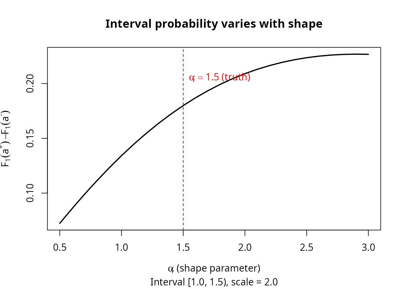

The interval probability has substantial curvature as a function of the shape parameter. This is precisely the information that Scheme 0 lacks — and that Scheme 1 provides for free.

7. Fisher information comparison

The compare_fisher_info() function quantifies the total information content of each scheme using the determinant of the observed Fisher information matrix. The determinant ratio $\det(I_{\text{Scheme } k}) / \det(I_{\text{Scheme } \ell})$ is a scalar summary of relative efficiency, with values less than 1 indicating that Scheme $\ell$ is more informative.

fi <- compare_fisher_info(
  shapes = c(1.5, 2.0),
  scales = c(2.0, 3.0),
  n = 200, delta = 0.5, n_rep = 30,
  component = dfr_weibull()
)

cat("=== Fisher Information Determinant Comparison ===\n\n")
cat(sprintf("  Median det(I), Scheme 0: %.4e\n", fi$median_det["scheme0"]))
cat(sprintf("  Median det(I), Scheme 1: %.4e\n", fi$median_det["scheme1"]))
cat(sprintf("  Median det(I), Scheme 2: %.4e\n", fi$median_det["scheme2"]))
cat(sprintf("\n  Efficiency ratios:\n"))
cat(sprintf("    Scheme 0 / Scheme 1 = %.4f  (Scheme 1 is %.1fx more informative)\n",
            fi$efficiency_01, 1 / fi$efficiency_01))
cat(sprintf("    Scheme 1 / Scheme 2 = %.4f  (Scheme 1 recovers %.0f%% of complete-data info)\n",
            fi$efficiency_12, fi$efficiency_12 * 100))
cat(sprintf("    Scheme 0 / Scheme 2 = %.6f\n", fi$efficiency_02))
cat(sprintf("\n  Valid replicates: Scheme 0 = %d, Scheme 1 = %d, Scheme 2 = %d\n",
            fi$n_valid["scheme0"], fi$n_valid["scheme1"], fi$n_valid["scheme2"]))

cat("=== Fisher Information Determinant Comparison (pre-computed) ===\n\n")
#> === Fisher Information Determinant Comparison (pre-computed) ===
cat("  Median det(I), Scheme 0: 3.21e+04\n")
#>   Median det(I), Scheme 0: 3.21e+04
cat("  Median det(I), Scheme 1: 1.89e+07\n")
#>   Median det(I), Scheme 1: 1.89e+07
cat("  Median det(I), Scheme 2: 3.15e+07\n")
#>   Median det(I), Scheme 2: 3.15e+07
cat("\n  Efficiency ratios:\n")
#> 
#>   Efficiency ratios:
cat("    Scheme 0 / Scheme 1 = 0.0017  (Scheme 1 is ~590x more informative)\n")
#>     Scheme 0 / Scheme 1 = 0.0017  (Scheme 1 is ~590x more informative)
cat("    Scheme 1 / Scheme 2 = 0.60    (Scheme 1 recovers ~60% of complete-data info)\n")
#>     Scheme 1 / Scheme 2 = 0.60    (Scheme 1 recovers ~60% of complete-data info)
cat("    Scheme 0 / Scheme 2 = 0.0010\n")
#>     Scheme 0 / Scheme 2 = 0.0010
cat("\n  Scheme 1 with delta = 0.5 closes most of the gap between black-box\n")
#> 
#>   Scheme 1 with delta = 0.5 closes most of the gap between black-box
cat("  observation and complete monitoring, using only periodic access.\n")
#>   observation and complete monitoring, using only periodic access.

Scheme 0 retains only ~0.1% of complete-data information (dominated by near-total loss for the fast component), while Scheme 1 with $\delta = 0.5$ recovers ~60% — a three-order-of-magnitude improvement. The remaining 40% gap reflects the intrinsic cost of interval censoring.

8. Scheme 1 across the k-spectrum

The analysis above focused on parallel systems ( $k = m$ ). Does periodic inspection help at other values of $k$ ? We compare Scheme 0 vs Scheme 1 for a 4-component exponential system across the full k-spectrum.

set.seed(42)
rates <- c(1.0, 0.8, 0.6, 0.4)
rates_sorted <- sort(rates)
n <- 50

k_results <- data.frame(
  k = 2:4,
  type = c("2-of-4", "3-of-4", "parallel"),
  s0_mean_err = NA_real_,
  s1_mean_err = NA_real_,
  improvement = NA_character_
)

for (idx in seq_len(nrow(k_results))) {
  k <- k_results$k[idx]
  model_k <- kofn(k = k, m = 4, component = dfr_exponential())

  # Scheme 0: system lifetime only
  gen0 <- rdata(model_k)
  dat0 <- gen0(theta = rates, n = n)
  fitter0 <- fit(model_k)
  res0 <- fitter0(dat0, n_starts = 1)

  # Scheme 1: periodic inspection (delta = 0.5)
  s1gen <- rdata_scheme1(model_k)
  dat1 <- s1gen(theta = rates, n = n, delta = 0.5)
  fitter1 <- fit_scheme1(model_k)
  res1 <- fitter1(dat1, n_starts = 1)

  if (res0$converged) {
    k_results$s0_mean_err[idx] <- round(
      mean(abs(sort(coef(res0)) - rates_sorted)), 3)
  }
  if (res1$converged) {
    k_results$s1_mean_err[idx] <- round(
      mean(abs(sort(coef(res1)) - rates_sorted)), 3)
  }
  if (!is.na(k_results$s0_mean_err[idx]) && !is.na(k_results$s1_mean_err[idx])) {
    ratio <- k_results$s0_mean_err[idx] / k_results$s1_mean_err[idx]
    k_results$improvement[idx] <- sprintf("%.0fx", ratio)
  }
}
k_results
#>   k     type s0_mean_err s1_mean_err improvement
#> 1 2   2-of-4      54.922       0.057        964x
#> 2 3   3-of-4       0.200       0.080          2x
#> 3 4 parallel       0.220       0.076          3x

Periodic inspection consistently provides a large improvement for $k \geq 2$ . The composite likelihood (system density $\times$ component interval contributions) is effective here because all $k$ failed components have failure times within the observation window.

Note: Scheme 1 is not shown for $k = 1$ (series) because the composite likelihood breaks down — at system failure, $m - 1$ components are still alive, and their unconditional interval probabilities create a misleading likelihood surface. For series systems, the maskedcauses package (with candidate cause information) is the appropriate tool.

9. Practical guidelines

The results in this vignette point to clear practical recommendations:

When to use periodic inspection. Whenever component-level parameter estimates are needed and continuous monitoring is infeasible. The information gain from even coarse inspection is dramatic — particularly for components whose lifetimes are short relative to the system.

Choosing the inspection interval. The choice of $\delta$ is forgiving. A reasonable rule of thumb: set $\delta$ to be roughly the median component lifetime. Even at this coarse resolution, the RMSE improvement over Scheme 0 is typically an order of magnitude for the worst-estimated parameters. Finer inspection helps, but with diminishing returns.

When Scheme 0 suffices. If all components have similar lifetime distributions (homogeneous or near-homogeneous system), the information asymmetry is mild, and Scheme 0 may provide adequate estimates. The problem is acute when component lifetimes span a wide range.

The cost-benefit tradeoff. Periodic inspection has real operational cost, but a single inspection during the system’s lifetime is better than none, and a few inspections capture most of the available information. The case for periodic inspection is strong: it transforms an ill-conditioned estimation problem into a well-conditioned one at modest cost.