Multivariate and Mixture Distributions • algebraic.dist

library(algebraic.dist)

This vignette covers the multivariate normal (MVN), affine transformations, and mixture distribution facilities in algebraic.dist. These features were introduced in version 0.3.0 and provide closed-form operations wherever possible, falling back to Monte Carlo only when necessary.

MVN Basics

Construct an MVN with mvn(). The mu argument is the mean vector and sigma is the variance-covariance matrix (defaulting to the identity).

M <- mvn(mu = c(1, 2, 3),
         sigma = matrix(c(1.0, 0.5, 0.2,
                          0.5, 2.0, 0.3,
                          0.2, 0.3, 1.5), nrow = 3, byrow = TRUE))
M
#> Multivariate normal distribution (3 dimensions) 
#>   mu:
#> [1] 1 2 3
#>   sigma:
#>      [,1] [,2] [,3]
#> [1,]  1.0  0.5  0.2
#> [2,]  0.5  2.0  0.3
#> [3,]  0.2  0.3  1.5

Standard accessors return the moments and dimensionality.

mean(M)
#> [1] 1 2 3
vcov(M)
#>      [,1] [,2] [,3]
#> [1,]  1.0  0.5  0.2
#> [2,]  0.5  2.0  0.3
#> [3,]  0.2  0.3  1.5
dim(M)
#> [1] 3

The params() generic flattens all parameters into a single named vector (useful for optimisation interfaces).

params(M)
#>    mu1    mu2    mu3 sigma1 sigma2 sigma3 sigma4 sigma5 sigma6 sigma7 sigma8 
#>    1.0    2.0    3.0    1.0    0.5    0.2    0.5    2.0    0.3    0.2    0.3 
#> sigma9 
#>    1.5

Sampling

sampler() returns a reusable sampling function. The output is an n-by-d matrix where rows are observations and columns are dimensions.

set.seed(42)
samp <- sampler(M)
X <- samp(100)
dim(X)
#> [1] 100   3
head(X, 5)
#>            [,1]     [,2]     [,3]
#> [1,]  2.2489225 1.535966 3.491808
#> [2,]  1.6922001 2.683528 2.965904
#> [3,]  2.6174451 2.400164 5.569057
#> [4,]  1.3945273 4.054878 5.919814
#> [5,] -0.4226174 1.308804 2.695016

Marginals

Extracting a marginal over a subset of indices returns a new MVN (or a univariate normal when a single index is selected).

M13 <- marginal(M, c(1, 3))
M13
#> Multivariate normal distribution (2 dimensions) 
#>   mu:
#> [1] 1 3
#>   sigma:
#>      [,1] [,2]
#> [1,]  1.0  0.2
#> [2,]  0.2  1.5
mean(M13)
#> [1] 1 3
vcov(M13)
#>      [,1] [,2]
#> [1,]  1.0  0.2
#> [2,]  0.2  1.5

Selecting a single component yields a univariate normal.

M1 <- marginal(M, 1)
M1
#> Normal distribution (mu = 1, var = 1)
mean(M1)
#> [1] 1
vcov(M1)
#> [1] 1

Closed-Form MVN Conditioning

Conditioning a multivariate normal on observed values uses the Schur complement formula. Given an MVN partitioned into free variables $X_1$ and observed variables $X_2 = a$ , the conditional distribution is:

$X_1 \mid X_2 = a \;\sim\; \mathcal{N}\!\bigl(\mu_1 + \Sigma_{12}\Sigma_{22}^{-1}(a - \mu_2),\;\; \Sigma_{11} - \Sigma_{12}\Sigma_{22}^{-1}\Sigma_{21}\bigr)$

This is exact – no Monte Carlo is involved.

M2 <- mvn(mu = c(0, 0), sigma = matrix(c(1, 0.8, 0.8, 1), 2, 2))

# Condition on X2 = 1
M_cond <- conditional(M2, given_indices = 2, given_values = 1)
mean(M_cond)
#> [1] 0.8
vcov(M_cond)
#> [1] 0.36

With $\rho = 0.8$ , the conditional mean is $\mu_1 + \rho(1 - \mu_2) = 0 + 0.8(1 - 0) = 0.8$ , and the conditional variance is $1 - \rho^2 = 1 - 0.64 = 0.36$ .

Predicate-based MC fallback

When the conditioning event is not “observe variable $j$ at value $a$ ” but an arbitrary predicate, the package falls back to Monte Carlo. This is accessed through the P argument.

set.seed(42)
M_cond_mc <- conditional(M2, P = function(x) abs(x[2] - 1) < 0.1)
mean(M_cond_mc)
#> [1] 0.7938476 0.9969783

The MC result is approximate and depends on the tolerance in the predicate. Prefer the closed-form interface whenever possible.

Affine Transformations

affine_transform(x, A, b) computes the distribution of $Y = AX + b$ where $X \sim \text{MVN}(\mu, \Sigma)$ . The result is:

$Y \sim \text{MVN}(A\mu + b,\;\; A \Sigma A^\top)$

This is a closed-form operation that returns a new MVN (or normal if the result is one-dimensional).

Portfolio example

Consider two assets with expected returns and a covariance structure. A portfolio is a linear combination of the returns.

returns <- mvn(
  mu = c(0.05, 0.08),
  sigma = matrix(c(0.04, 0.01,
                   0.01, 0.09), 2, 2)
)

# 60/40 portfolio weights
w <- matrix(c(0.6, 0.4), nrow = 1)
portfolio <- affine_transform(returns, A = w)
mean(portfolio)
#> [1] 0.062
vcov(portfolio)
#> [1] 0.0336

The portfolio return is $0.6 \times 0.05 + 0.4 \times 0.08 = 0.062$ . The portfolio variance is $w \Sigma w^\top$ , a scalar that captures the diversification benefit.

Dimensionality reduction

Affine transforms can also project to lower dimensions. For instance, computing the sum and difference of two variables.

X <- mvn(mu = c(3, 7), sigma = matrix(c(4, 1, 1, 9), 2, 2))

# A maps (X1, X2) -> (X1 + X2, X1 - X2)
A <- matrix(c(1, 1,
              1, -1), nrow = 2, byrow = TRUE)
Y <- affine_transform(X, A = A)
mean(Y)
#> [1] 10 -4
vcov(Y)
#>      [,1] [,2]
#> [1,]   15   -5
#> [2,]   -5   11

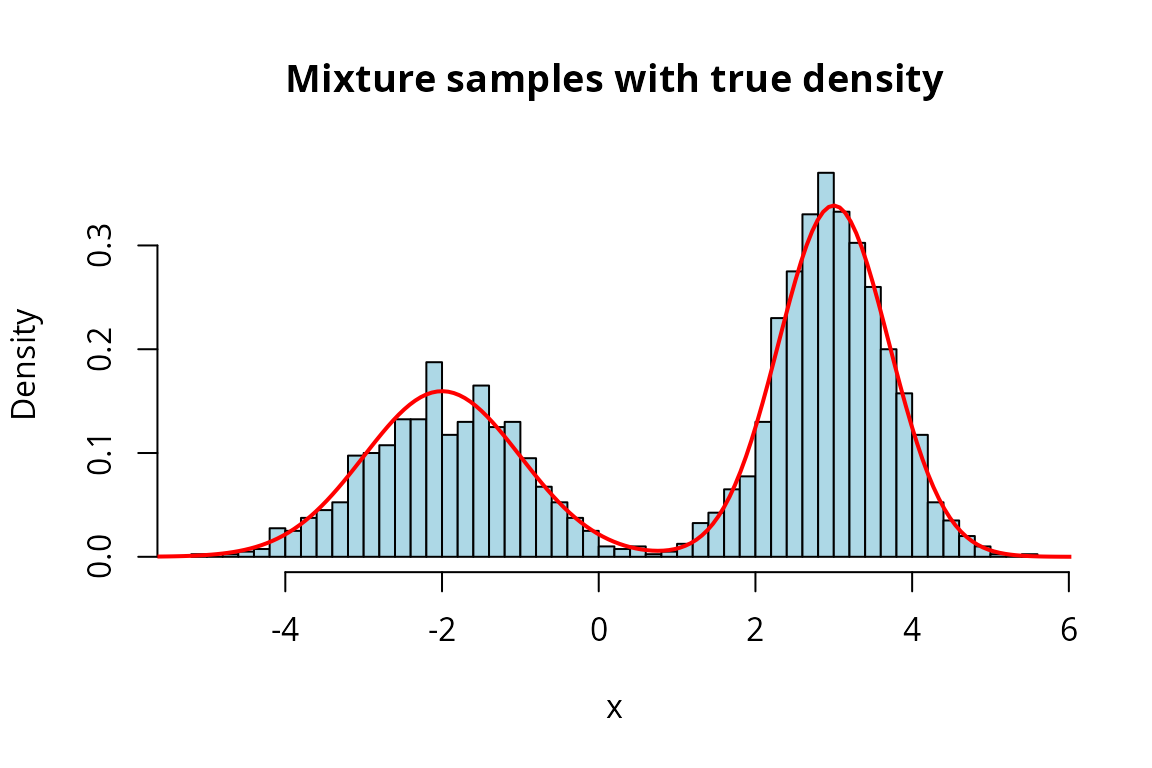
Mixture Distribution Basics

A mixture distribution is constructed from a list of component distributions and a vector of non-negative weights that sum to one.

m <- mixture(
  components = list(normal(-2, 1), normal(3, 0.5)),
  weights = c(0.4, 0.6)
)
m
#> Mixture distribution (2 components) 
#>   [w=0.400] Normal distribution (mu = -2, var = 1)
#>   [w=0.600] Normal distribution (mu = 3, var = 0.5)

Mean and variance

The mixture mean is the weighted average of component means: $E[X] = \sum_k w_k \mu_k$ .

mean(m)
#> [1] 1

The mixture variance uses the law of total variance: $\text{Var}(X) = \underbrace{\sum_k w_k \sigma_k^2}_{\text{within-component}} + \underbrace{\sum_k w_k(\mu_k - \bar\mu)^2}_{\text{between-component}}$ .

vcov(m)
#> [1] 6.7

The between-component term captures the spread of the component means around the overall mean. This is why mixtures can have much larger variance than any individual component.

Density and CDF

density() and cdf() return callable functions, following the same pattern as other distributions in the package.

f <- density(m)

x_vals <- seq(-6, 8, length.out = 200)
y_vals <- sapply(x_vals, f)
plot(x_vals, y_vals, type = "l", lwd = 2,
     main = "Bimodal mixture density",
     xlab = "x", ylab = "f(x)")

The bimodal shape is clearly visible, with peaks near $-2$ and $3$ .

F <- cdf(m)
F_vals <- sapply(x_vals, F)
plot(x_vals, F_vals, type = "l", lwd = 2,
     main = "Mixture CDF",
     xlab = "x", ylab = "F(x)")

Sampling

set.seed(123)
s <- sampler(m)
samples <- s(2000)
hist(samples, breaks = 50, probability = TRUE, col = "lightblue",
     main = "Mixture samples with true density",
     xlab = "x")
lines(x_vals, y_vals, col = "red", lwd = 2)

Mixture Operations

Marginals of mixtures

The marginal of a mixture is a mixture of marginals with the same weights. This follows directly from the definition: $p(x_I) = \sum_k w_k\, p_k(x_I)$ .

m2 <- mixture(
  list(mvn(c(0, 0), diag(2)), mvn(c(3, 3), diag(2))),
  c(0.5, 0.5)
)

m2_x1 <- marginal(m2, 1)
m2_x1
#> Mixture distribution (2 components) 
#>   [w=0.500] Normal distribution (mu = 0, var = 1)
#>   [w=0.500] Normal distribution (mu = 3, var = 1)
mean(m2_x1)
#> [1] 1.5

The marginal mean is $0.5 \times 0 + 0.5 \times 3 = 1.5$ , the weighted average of the component marginal means.

Conditional of mixtures (Bayesian weight update)

Conditioning a mixture on observed values updates the component weights via Bayes’ rule. Each component’s weight is scaled by its marginal density at the observed value:

$w_k' \propto w_k \, f_k(x_{\text{obs}})$

Components whose marginal density is higher at the observed value receive more weight.

mc <- conditional(m2, given_indices = 2, given_values = 0)
mc
#> Mixture distribution (2 components) 
#>   [w=0.989] Normal distribution (mu = 0, var = 1)
#>   [w=0.011] Normal distribution (mu = 3, var = 1)
mean(mc)
#> [1] 0.03296083

Conditioning on $X_2 = 0$ shifts weight toward the first component (whose mean for $X_2$ is 0) and away from the second component (whose mean for $X_2$ is 3). The conditional mean of $X_1$ is therefore pulled closer to 0 than the unconditional value of 1.5.

We can also condition at a value near the second component to see the opposite effect.

mc_high <- conditional(m2, given_indices = 2, given_values = 3)
mc_high
#> Mixture distribution (2 components) 
#>   [w=0.011] Normal distribution (mu = 0, var = 1)
#>   [w=0.989] Normal distribution (mu = 3, var = 1)
mean(mc_high)
#> [1] 2.967039

Now the weight shifts toward the second component, and the conditional mean of $X_1$ is pulled toward 3.

Practical Example: Gaussian Mixture Classification

Gaussian mixture models (GMMs) are widely used for soft classification. The idea: each component represents a class, and conditioning on observed features updates the class probabilities.

Setup: a two-class GMM

Consider two clusters in 2D, representing two classes with equal prior probability.

class_a <- mvn(c(-2, -1), matrix(c(1.0, 0.3, 0.3, 0.8), 2, 2))
class_b <- mvn(c(2, 1.5), matrix(c(0.6, -0.2, -0.2, 1.2), 2, 2))

gmm <- mixture(
  components = list(class_a, class_b),
  weights = c(0.5, 0.5)
)
gmm
#> Mixture distribution (2 components) 
#>   [w=0.500] Multivariate normal distribution (2 dimensions)
#>   [w=0.500] Multivariate normal distribution (2 dimensions)

Visualise the clusters

set.seed(314)
samp_a <- sampler(class_a)(300)
samp_b <- sampler(class_b)(300)

plot(samp_a[, 1], samp_a[, 2], col = "steelblue", pch = 16, cex = 0.6,
     xlim = c(-6, 6), ylim = c(-5, 5),
     xlab = expression(X[1]), ylab = expression(X[2]),
     main = "Two-class GMM samples")
points(samp_b[, 1], samp_b[, 2], col = "tomato", pch = 16, cex = 0.6)
legend("topright", legend = c("Class A", "Class B"),
       col = c("steelblue", "tomato"), pch = 16)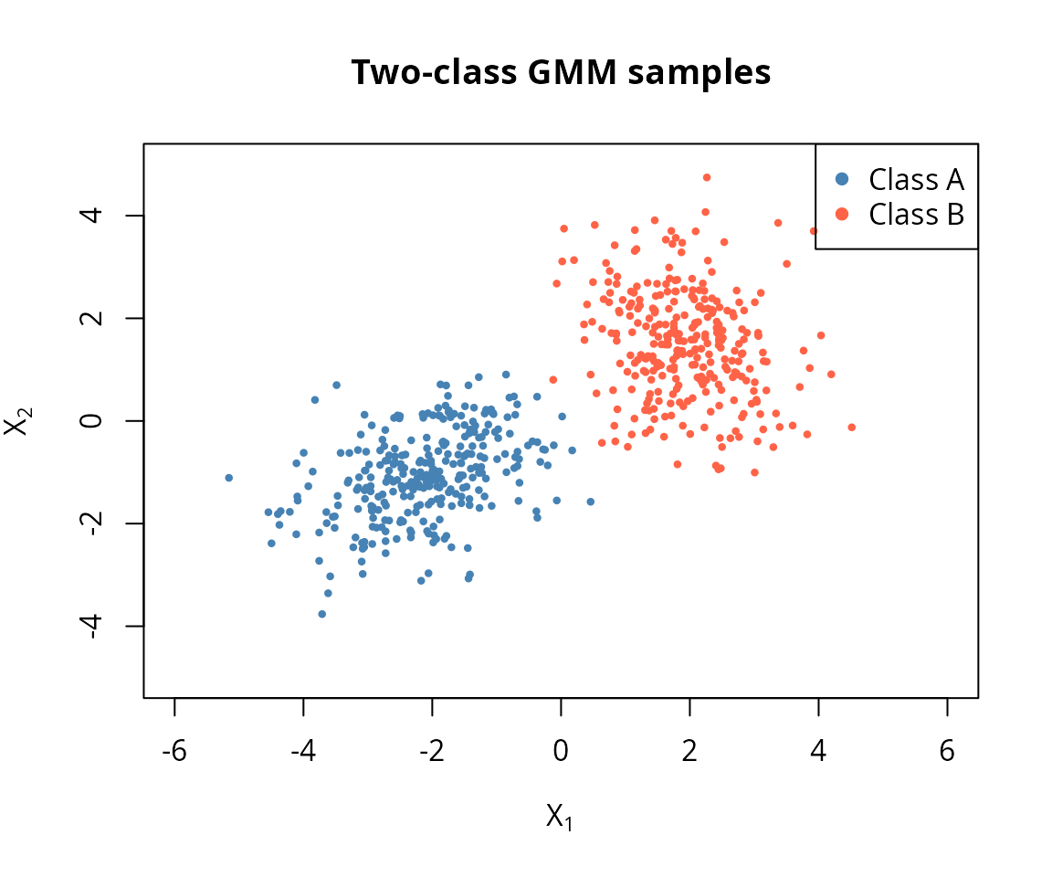

Soft classification by conditioning

Suppose we observe $X_1 = -1$ . Conditioning updates the class weights based on how likely each component is to produce that value.

post_neg <- conditional(gmm, given_indices = 1, given_values = -1)
post_neg
#> Mixture distribution (2 components) 
#>   [w=0.999] Normal distribution (mu = -0.7, var = 0.71)
#>   [w=0.001] Normal distribution (mu = 2.5, var = 1.13333)

The updated weights give the posterior class probabilities. Since $X_1 = -1$ is much more likely under Class A (centred at $-2$ ) than Class B (centred at $2$ ), Class A receives most of the weight.

The conditional distribution of $X_2$ given $X_1 = -1$ is itself a mixture of the two conditional normals.

f_post <- density(post_neg)
x2_grid <- seq(-5, 5, length.out = 200)
y_post <- sapply(x2_grid, f_post)
plot(x2_grid, y_post, type = "l", lwd = 2,
     xlab = expression(X[2]),
     ylab = expression(f(X[2] ~ "|" ~ X[1] == -1)),
     main = "Posterior density of X2 given X1 = -1")

Now observe $X_1 = 2$ , which sits near the centre of Class B.

post_pos <- conditional(gmm, given_indices = 1, given_values = 2)
post_pos
#> Mixture distribution (2 components) 
#>   [w=0.000] Normal distribution (mu = 0.2, var = 0.71)
#>   [w=1.000] Normal distribution (mu = 1.5, var = 1.13333)

As expected, the weight shifts heavily toward Class B. The conditional density of $X_2$ now concentrates around the Class B conditional mean.

f_post_pos <- density(post_pos)
y_post_pos <- sapply(x2_grid, f_post_pos)
plot(x2_grid, y_post_pos, type = "l", lwd = 2,
     xlab = expression(X[2]),
     ylab = expression(f(X[2] ~ "|" ~ X[1] == 2)),
     main = "Posterior density of X2 given X1 = 2")

Ambiguous observations

When the observation falls between the two cluster means, both classes retain meaningful probability and the posterior becomes bimodal.

post_mid <- conditional(gmm, given_indices = 1, given_values = 0)
post_mid
#> Mixture distribution (2 components) 
#>   [w=0.746] Normal distribution (mu = -0.4, var = 0.71)
#>   [w=0.254] Normal distribution (mu = 2.16667, var = 1.13333)

f_post_mid <- density(post_mid)
y_post_mid <- sapply(x2_grid, f_post_mid)
plot(x2_grid, y_post_mid, type = "l", lwd = 2,
     xlab = expression(X[2]),
     ylab = expression(f(X[2] ~ "|" ~ X[1] == 0)),
     main = "Posterior density of X2 given X1 = 0 (ambiguous)")

At $X_1 = 0$ the posterior for $X_2$ is bimodal – one mode near the Class A conditional mean, one near Class B. Although $X_1 = 0$ is equidistant from the two class means ( $-2$ and $2$ ), Class A receives roughly 75% of the posterior weight because its broader $X_1$ variance ( $\sigma^2 = 1$ vs $0.6$ ) gives it higher density at the midpoint. Class B still retains about 25% of the weight, so neither class is overwhelmingly dominant. This is the hallmark of soft classification: rather than forcing a hard decision, the mixture posterior represents genuine uncertainty about the class label.