Theory and Intuition Behind Numerical MLE

Alexander Towell

2025-12-02

What is Maximum Likelihood Estimation?

Maximum Likelihood Estimation (MLE) is a fundamental method for estimating the parameters of a statistical model. The idea is simple yet powerful: find the parameter values that make the observed data most probable.

The Likelihood Function

Suppose we observe data $x_1, x_2, \ldots, x_n$ and we believe it comes from a probability distribution with parameter(s) $\theta$. The likelihood function $L(\theta)$ measures how probable the observed data is, given parameter $\theta$:

$$L(\theta) = P(X_1 = x_1, X_2 = x_2, \ldots, X_n = x_n \mid \theta)$$

For independent observations:

$$L(\theta) = \prod_{i=1}^{n} f(x_i \mid \theta)$$

where $f(\cdot \mid \theta)$ is the probability density (or mass) function.

Why Log-Likelihood?

Working with products is numerically unstable and mathematically inconvenient. Taking the logarithm converts products to sums:

$$\ell(\theta) = \log L(\theta) = \sum_{i=1}^{n} \log f(x_i \mid \theta)$$

Since $\log$ is monotonic, maximizing $\ell(\theta)$ is equivalent to maximizing $L(\theta)$. The log-likelihood has several advantages:

1. Numerical stability: Products of small probabilities can underflow to zero
2. Computational efficiency: Sums are faster than products
3. Mathematical convenience: Derivatives of sums are easier than derivatives of products
4. Statistical properties: The curvature of $\ell(\theta)$ relates to estimation uncertainty

A Concrete Example

Let’s see this with normal data:

set.seed(42)
x <- rnorm(50, mean = 3, sd = 1.5)

# Log-likelihood function for normal distribution
loglike <- function(theta) {
  mu <- theta[1]
  sigma <- theta[2]
  if (sigma <= 0) return(-Inf)
  sum(dnorm(x, mean = mu, sd = sigma, log = TRUE))
}

# Visualize the log-likelihood surface
mu_grid <- seq(1, 5, length.out = 50)
sigma_grid <- seq(0.5, 3, length.out = 50)
ll_surface <- outer(mu_grid, sigma_grid, function(m, s) {
  mapply(function(mi, si) loglike(c(mi, si)), m, s)
})

# Contour plot
contour(mu_grid, sigma_grid, ll_surface, nlevels = 20,
        xlab = expression(mu), ylab = expression(sigma),
        main = "Log-Likelihood Surface")
points(mean(x), sd(x), pch = 19, col = "red", cex = 1.5)
legend("topright", "MLE", pch = 19, col = "red")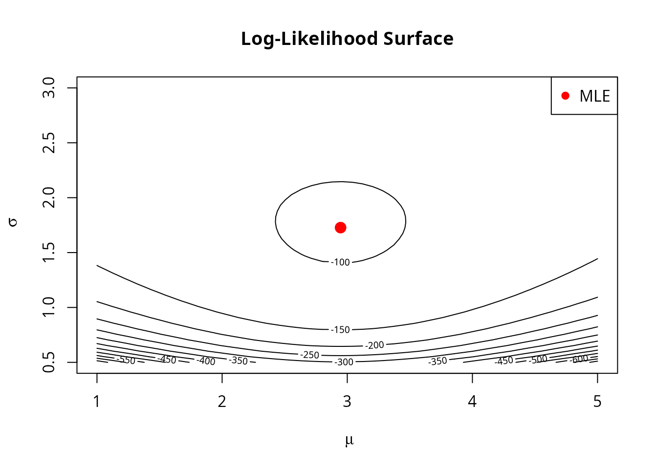

The MLE is the point on this surface with the highest value (deepest red in the contour plot).

The Score Function

The score function is the gradient (vector of partial derivatives) of the log-likelihood:

$$s(\theta) = \nabla_\theta \ell(\theta) = \left( \frac{\partial \ell}{\partial \theta_1}, \ldots, \frac{\partial \ell}{\partial \theta_p} \right)$$

At the MLE $\hat{\theta}$, the score is zero: $s(\hat{\theta}) = 0$.

Intuition

The score tells us the direction of steepest ascent on the log-likelihood surface. If $s(\theta) \neq 0$, we can increase the likelihood by moving in the direction of $s(\theta)$.

# Score function for normal distribution
score <- function(theta) {
  mu <- theta[1]
  sigma <- theta[2]
  n <- length(x)
  c(
    sum(x - mu) / sigma^2,                        # d/d_mu
    -n / sigma + sum((x - mu)^2) / sigma^3        # d/d_sigma
  )
}

# At a point away from the MLE, the score points toward the MLE
theta_start <- c(1, 0.8)
s <- score(theta_start)
cat("Score at (1, 0.8):", round(s, 2), "\n")
#> Score at (1, 0.8): 152.07 593.01
cat("Direction: move", ifelse(s[1] > 0, "right", "left"), "in mu,",
    ifelse(s[2] > 0, "up", "down"), "in sigma\n")
#> Direction: move right in mu, up in sigma

Gradient Ascent

Gradient ascent is the simplest optimization algorithm. It iteratively moves in the direction of the gradient:

$$\theta^{(t+1)} = \theta^{(t)} + \eta \cdot s(\theta^{(t)})$$

where $\eta > 0$ is the learning rate (step size).

Why It Works

The score points in the direction of steepest increase. Taking small steps in this direction guarantees improvement (for small enough $\eta$).

The Challenge: Choosing the Step Size

• Too large: We might overshoot and oscillate
• Too small: Convergence is painfully slow

# Demonstrate gradient ascent with different step sizes
run_gradient_ascent <- function(eta, max_iter = 50) {
  theta <- c(1, 0.8)
  path <- matrix(NA, max_iter + 1, 2)
  path[1, ] <- theta

  for (i in 1:max_iter) {
    theta <- theta + eta * score(theta)
    if (theta[2] <= 0) theta[2] <- 0.01  # Enforce constraint
    path[i + 1, ] <- theta
  }
  path
}

# Compare step sizes
path_small <- run_gradient_ascent(0.001)
path_good <- run_gradient_ascent(0.01)
path_large <- run_gradient_ascent(0.05)

# Plot paths
contour(mu_grid, sigma_grid, ll_surface, nlevels = 15,
        xlab = expression(mu), ylab = expression(sigma),
        main = "Gradient Ascent: Effect of Step Size")
lines(path_small[, 1], path_small[, 2], col = "blue", lwd = 2)
lines(path_good[, 1], path_good[, 2], col = "green", lwd = 2)
lines(path_large[1:20, 1], path_large[1:20, 2], col = "red", lwd = 2)
points(mean(x), sd(x), pch = 19, cex = 1.5)
legend("topright", c("Small (0.001)", "Good (0.01)", "Large (0.05)"),
       col = c("blue", "green", "red"), lwd = 2)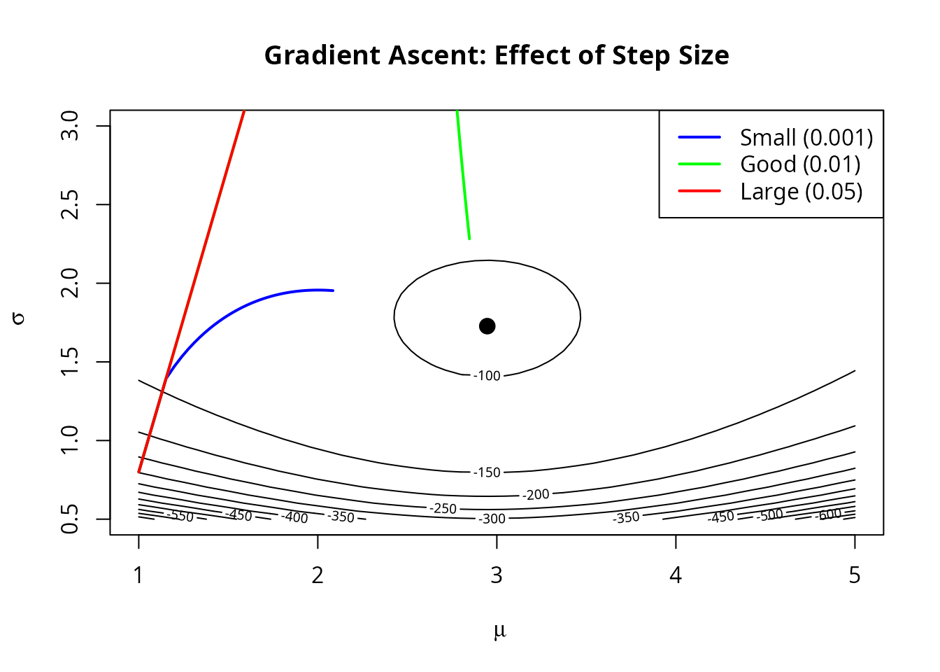

Line Search: Automatic Step Size Selection

Backtracking line search adaptively finds a good step size:

1. Start with a large step size
2. If it doesn’t improve the objective enough, shrink it
3. Repeat until we find an acceptable step

This is implemented in mle_config_linesearch():

result <- mle_gradient_ascent(
  loglike = loglike,
  score = score,
  theta0 = c(1, 0.8),
  config = mle_config_linesearch(max_iter = 50, trace = TRUE),
  constraint = mle_constraint(
    support = function(theta) theta[2] > 0,
    project = function(theta) c(theta[1], max(theta[2], 1e-6))
  )
)

cat("Final estimate:", round(result$theta.hat, 4), "\n")
#> Final estimate: 2.9472 1.7103
cat("Iterations:", result$iter, "\n")
#> Iterations: 8
cat("Converged:", result$converged, "\n")
#> Converged: FALSE

The Fisher Information Matrix

The Fisher information matrix $I(\theta)$ measures how much information the data carries about $\theta$:

$$I(\theta) = -E\left[ \frac{\partial^2 \ell}{\partial \theta \partial \theta^T} \right]$$

It’s also related to the variance of the score: $I(\theta) = \text{Var}(s(\theta))$.

Why It Matters

1. Curvature: $I(\theta)$ describes the curvature of the log-likelihood surface
2. Uncertainty: The inverse $I(\theta)^{-1}$ approximates the covariance of $\hat{\theta}$
3. Natural scaling: Different parameters may have different scales; $I(\theta)$ accounts for this

Observed vs Expected Fisher Information

• Expected information: $I(\theta) = -E[\nabla^2 \ell(\theta)]$
• Observed information: $J(\theta) = -\nabla^2 \ell(\theta)$ (evaluated at the data)

In practice, we often use the observed information, which doesn’t require computing expectations.

Newton-Raphson

Newton-Raphson uses the Fisher information to take smarter steps:

$$\theta^{(t+1)} = \theta^{(t)} + I(\theta^{(t)})^{-1} s(\theta^{(t)})$$

Intuition

Gradient ascent treats all directions equally, but some directions might be “easier” to move in than others. Newton-Raphson pre-multiplies by $I^{-1}$, which:

• Takes larger steps in flat directions (low curvature)
• Takes smaller steps in curved directions (high curvature)
• Accounts for correlations between parameters

Comparison

# Fisher information for normal distribution
fisher <- function(theta) {
  sigma <- theta[2]
  n <- length(x)
  matrix(c(
    n / sigma^2, 0,
    0, 2 * n / sigma^2
  ), nrow = 2)
}

# Run gradient ascent
result_ga <- mle_gradient_ascent(
  loglike = loglike,
  score = score,
  theta0 = c(1, 0.8),
  config = mle_config_linesearch(max_iter = 100, trace = TRUE),
  constraint = mle_constraint(
    support = function(theta) theta[2] > 0,
    project = function(theta) c(theta[1], max(theta[2], 1e-6))
  )
)

# Run Newton-Raphson
result_nr <- mle_newton_raphson(
  loglike = loglike,
  score = score,
  fisher = fisher,
  theta0 = c(1, 0.8),
  config = mle_config_linesearch(max_iter = 100, trace = TRUE),
  constraint = mle_constraint(
    support = function(theta) theta[2] > 0,
    project = function(theta) c(theta[1], max(theta[2], 1e-6))
  )
)

cat("Gradient Ascent: ", result_ga$iter, "iterations\n")
#> Gradient Ascent:  8 iterations
cat("Newton-Raphson:  ", result_nr$iter, "iterations\n")
#> Newton-Raphson:   11 iterations

Newton-Raphson typically converges much faster, especially near the optimum where its quadratic convergence kicks in.

When to Use Which Method

Use Gradient Ascent When:

• You don’t have (or can’t easily compute) the Fisher information
• The problem is high-dimensional (computing $I^{-1}$ is expensive)
• You’re using stochastic gradients (mini-batches)
• Getting a rough answer quickly is acceptable

Use Newton-Raphson When:

• You need high precision
• The Fisher information is available and cheap to compute
• The problem is low-to-moderate dimensional
• Fast convergence is important

Use Grid Search When:

• The parameter space is small (1-3 dimensions)
• You need a good starting point
• The likelihood surface might have multiple modes

Use Random Restart When:

• The likelihood surface has multiple local maxima
• You’re uncertain about good starting values
• Robustness is more important than speed

Constrained Optimization

Real problems often have constraints on parameters:

• Variance must be positive: $\sigma > 0$
• Probabilities must be in $[0, 1]$
• Correlation must satisfy $|\rho| < 1$

Projection Method

The numerical.mle package uses projection: if a step takes us outside the feasible region, we project back to the nearest feasible point.

# Without constraint: optimization might fail
constraint <- mle_constraint(
  support = function(theta) theta[2] > 0,
  project = function(theta) c(theta[1], max(theta[2], 1e-6))
)

# The constraint keeps sigma positive throughout optimization
result <- mle_gradient_ascent(
  loglike = loglike,
  score = score,
  theta0 = c(0, 0.1),  # Start near the boundary
  config = mle_config_linesearch(max_iter = 100),
  constraint = constraint
)

cat("Final sigma:", result$theta.hat[2], "> 0 (constraint satisfied)\n")
#> Final sigma: 1.710644 > 0 (constraint satisfied)

Regularization and Penalized Likelihood

Sometimes we want to penalize certain parameter values to:

• Prevent overfitting
• Encourage sparsity
• Incorporate prior beliefs

Penalized Log-Likelihood

$$\ell_\lambda(\theta) = \ell(\theta) - \lambda \cdot P(\theta)$$

where $P(\theta)$ is a penalty function and $\lambda > 0$ controls regularization strength.

Common Penalties

L1 (LASSO): $P(\theta) = \sum_j |\theta_j|$

• Encourages sparsity (some $\theta_j = 0$)
• Useful for variable selection

L2 (Ridge): $P(\theta) = \sum_j \theta_j^2$

• Shrinks parameters toward zero
• Prevents extreme values
• Equivalent to Gaussian prior

Elastic Net: $P(\theta) = \alpha \sum_j |\theta_j| + (1-\alpha) \sum_j \theta_j^2$

• Combines L1 and L2 benefits
• $\alpha$ controls the mix

# Original log-likelihood (maximum at theta = 0)
loglike <- function(theta) -sum((theta - c(3, 2))^2)

# Add L2 penalty
loglike_l2 <- with_penalty(loglike, penalty_l2(), lambda = 1)

# Compare
theta <- c(3, 2)
cat("At theta = (3, 2):\n")
#> At theta = (3, 2):
cat("  Original:", loglike(theta), "\n")
#>   Original: 0
cat("  With L2 penalty:", loglike_l2(theta), "\n")
#>   With L2 penalty: -13
cat("  The penalty shrinks the solution toward zero\n")
#>   The penalty shrinks the solution toward zero

Stochastic Gradient Methods

For large datasets, computing the full gradient is expensive. Stochastic gradient ascent uses random subsamples:

$$\theta^{(t+1)} = \theta^{(t)} + \eta \cdot \hat{s}(\theta^{(t)})$$

where $\hat{s}$ is computed on a mini-batch of data.

Properties

• Noisy but unbiased: On average, we move in the right direction
• Faster iterations: Each step is cheap
• Implicit regularization: Noise can help escape local optima
• Requires care: Learning rate schedules, momentum, etc.

# Concept demonstration (not run)
loglike_full <- function(theta, obs = large_data) {
  sum(dnorm(obs, theta[1], theta[2], log = TRUE))
}

# Use only 100 observations per iteration
loglike_mini <- with_subsampling(
  loglike_full,
  data = large_data,
  subsample_size = 100
)

Convergence Criteria

The package checks for convergence using:

1. Absolute tolerance: $|\ell(\theta^{(t+1)}) - \ell(\theta^{(t)})| < \epsilon_{abs}$
2. Relative tolerance: $\frac{|\ell(\theta^{(t+1)}) - \ell(\theta^{(t)})|}{|\ell(\theta^{(t)})|} < \epsilon_{rel}$
3. Parameter change: $\|\theta^{(t+1)} - \theta^{(t)}\| < \epsilon$
4. Maximum iterations: Safety stop

config <- mle_config(
  max_iter = 500,     # Don't run forever
  abs_tol = 1e-8,     # Absolute change threshold
  rel_tol = 1e-6,     # Relative change threshold
  debug = FALSE       # Set TRUE to see iteration progress
)

Summary

Method	Order	Information Needed	Best For
Gradient Ascent	1st	Score only	Large problems, rough estimates
Newton-Raphson	2nd	Score + Fisher	High precision, small problems
Grid Search	0th	Likelihood only	Finding starting points
Random Restart	-	Varies	Multi-modal problems

The numerical.mle package provides a unified interface to all these methods, with composable configuration objects and function transformers to handle real-world complexities like constraints, regularization, and large datasets.

Further Reading

1. Casella, G. and Berger, R.L. (2002). Statistical Inference. Duxbury.
2. Nocedal, J. and Wright, S.J. (2006). Numerical Optimization. Springer.
3. Murphy, K.P. (2012). Machine Learning: A Probabilistic Perspective. MIT Press.