Case Studies: MLE for Common Distributions

Introduction

This vignette demonstrates using numerical.mle to fit various probability distributions to data. Each case study includes:

The log-likelihood and score functions
Appropriate constraints
Comparison with analytical solutions (where available)
Practical considerations

Case Study 1: Exponential Distribution

The exponential distribution is useful for modeling waiting times and lifetimes. It has one parameter: rate $\lambda > 0$ .

Setup

# Generate data
n <- 100
true_rate <- 2.5
x_exp <- rexp(n, rate = true_rate)

# Log-likelihood: sum of log(lambda * exp(-lambda * x))
loglike_exp <- function(lambda) {
  if (lambda <= 0) return(-Inf)
  n * log(lambda) - lambda * sum(x_exp)
}

# Score: d/d_lambda of log-likelihood
score_exp <- function(lambda) {
  n / lambda - sum(x_exp)
}

# Constraint: lambda must be positive
constraint_exp <- mle_constraint(
  support = function(lambda) lambda > 0,
  project = function(lambda) max(lambda, 1e-8)
)

Fitting

result_exp <- mle_gradient_ascent(
  loglike = loglike_exp,
  score = score_exp,
  theta0 = 1,
  config = mle_config_linesearch(max_iter = 50),
  constraint = constraint_exp
)

# Compare with analytical MLE: 1/mean(x)
mle_analytical <- 1 / mean(x_exp)

cat("Numerical MLE:   ", round(result_exp$theta.hat, 4), "\n")
#> Numerical MLE:    2.2227
cat("Analytical MLE:  ", round(mle_analytical, 4), "\n")
#> Analytical MLE:   2.2236
cat("True rate:       ", true_rate, "\n")
#> True rate:        2.5
cat("Iterations:      ", result_exp$iter, "\n")
#> Iterations:       6

Visualization

lambda_grid <- seq(0.1, 5, length.out = 100)
ll_values <- sapply(lambda_grid, loglike_exp)

plot(lambda_grid, ll_values, type = "l", lwd = 2,
     xlab = expression(lambda), ylab = "Log-likelihood",
     main = "Exponential Distribution Log-Likelihood")
abline(v = result_exp$theta.hat, col = "red", lwd = 2, lty = 2)
abline(v = true_rate, col = "blue", lwd = 2, lty = 3)
legend("topright", c("MLE", "True"), col = c("red", "blue"), lty = c(2, 3), lwd = 2)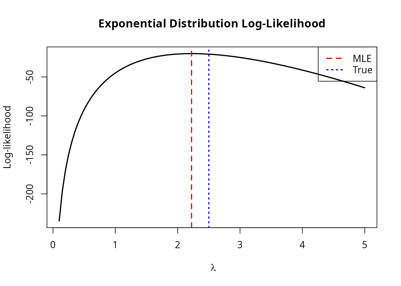

Case Study 2: Gamma Distribution

The gamma distribution generalizes the exponential with two parameters: shape $\alpha > 0$ and rate $\beta > 0$ .

Setup

# Generate data
true_shape <- 3
true_rate <- 2
x_gamma <- rgamma(200, shape = true_shape, rate = true_rate)

# Log-likelihood
loglike_gamma <- function(theta) {
  alpha <- theta[1]
  beta <- theta[2]
  if (alpha <= 0 || beta <= 0) return(-Inf)
  n <- length(x_gamma)
  n * (alpha * log(beta) - lgamma(alpha)) +
    (alpha - 1) * sum(log(x_gamma)) - beta * sum(x_gamma)
}

# Score function
score_gamma <- function(theta) {
  alpha <- theta[1]
  beta <- theta[2]
  n <- length(x_gamma)
  c(
    n * (log(beta) - digamma(alpha)) + sum(log(x_gamma)),  # d/d_alpha
    n * alpha / beta - sum(x_gamma)                         # d/d_beta
  )
}

# Both parameters must be positive
constraint_gamma <- mle_constraint(
  support = function(theta) all(theta > 0),
  project = function(theta) pmax(theta, 1e-6)
)

Fitting with Different Methods

# Gradient ascent
result_ga <- mle_gradient_ascent(
  loglike = loglike_gamma,
  score = score_gamma,
  theta0 = c(1, 1),
  config = mle_config_linesearch(max_iter = 200),
  constraint = constraint_gamma
)

# Grid search to find better starting point
result_grid <- mle_grid_search(
  loglike = loglike_gamma,
  lower = c(0.5, 0.5),
  upper = c(10, 10),
  grid_size = 20
)

# Refine with gradient ascent
result_refined <- mle_gradient_ascent(
  loglike = loglike_gamma,
  score = score_gamma,
  theta0 = result_grid$theta.hat,
  config = mle_config_linesearch(max_iter = 100),
  constraint = constraint_gamma
)

cat("Direct gradient ascent:\n")
#> Direct gradient ascent:
cat("  Shape:", round(result_ga$theta.hat[1], 4),
    " Rate:", round(result_ga$theta.hat[2], 4), "\n")
#>   Shape: 2.6637  Rate: 1.8497
cat("  Iterations:", result_ga$iter, "\n\n")
#>   Iterations: 38

cat("Grid search + refinement:\n")
#> Grid search + refinement:
cat("  Shape:", round(result_refined$theta.hat[1], 4),
    " Rate:", round(result_refined$theta.hat[2], 4), "\n")
#>   Shape: 2.6668  Rate: 1.8525
cat("  Iterations:", result_refined$iter, "(after grid)\n\n")
#>   Iterations: 60 (after grid)

cat("True parameters:\n")
#> True parameters:
cat("  Shape:", true_shape, " Rate:", true_rate, "\n")
#>   Shape: 3  Rate: 2

Visualization

# Create contour plot
alpha_grid <- seq(1, 6, length.out = 50)
beta_grid <- seq(0.5, 4, length.out = 50)
ll_gamma <- outer(alpha_grid, beta_grid, function(a, b) {
  mapply(function(ai, bi) loglike_gamma(c(ai, bi)), a, b)
})

contour(alpha_grid, beta_grid, ll_gamma, nlevels = 20,
        xlab = expression(alpha ~ "(shape)"),
        ylab = expression(beta ~ "(rate)"),
        main = "Gamma Distribution Log-Likelihood")
points(result_refined$theta.hat[1], result_refined$theta.hat[2],
       pch = 19, col = "red", cex = 1.5)
points(true_shape, true_rate, pch = 4, col = "blue", cex = 1.5, lwd = 2)
legend("topright", c("MLE", "True"), pch = c(19, 4), col = c("red", "blue"))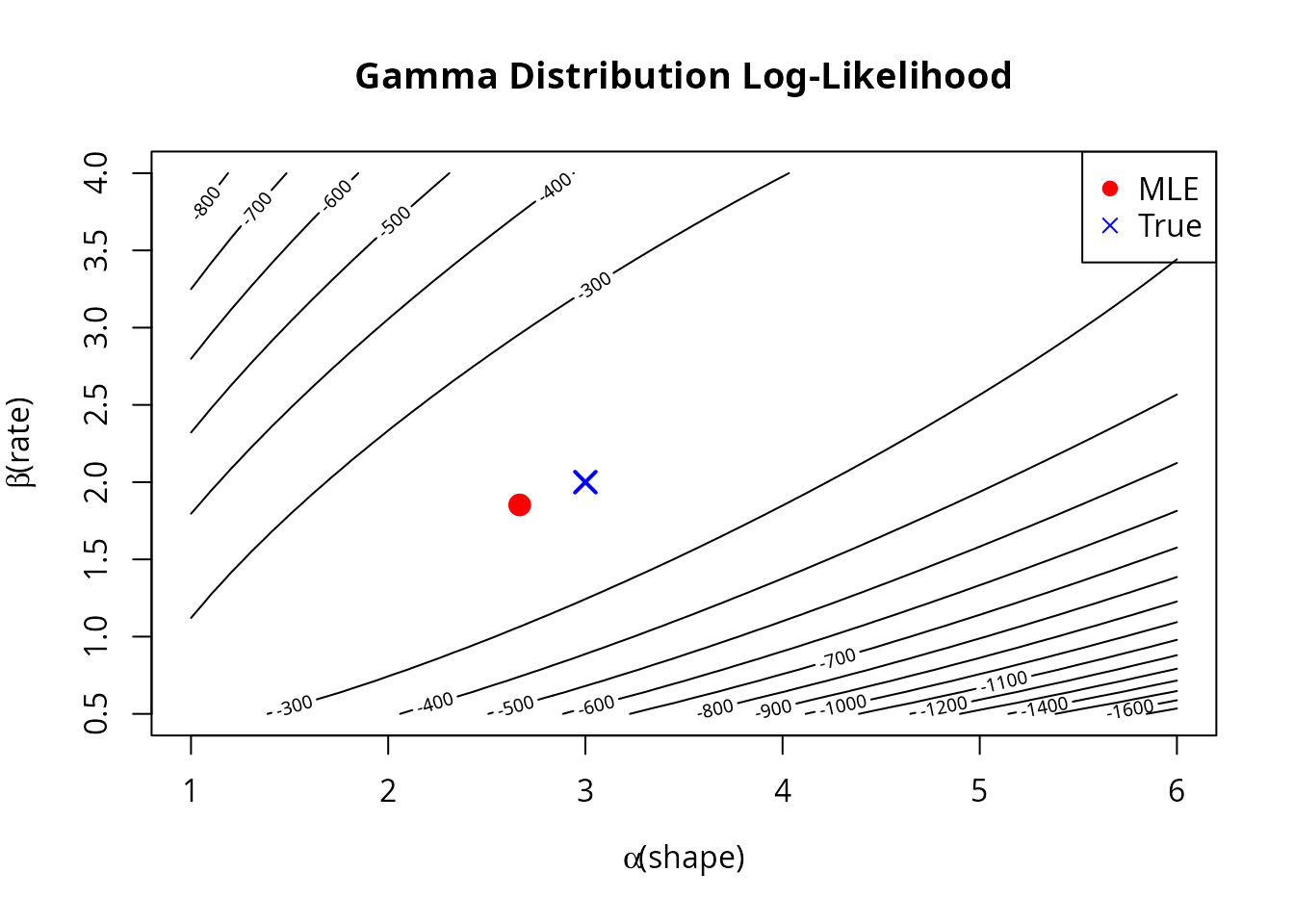

Case Study 3: Beta Distribution

The beta distribution is bounded on $[0, 1]$ and is useful for modeling proportions. It has shape parameters $\alpha > 0$ and $\beta > 0$ .

Setup

# Generate data
true_alpha <- 2
true_beta <- 5
x_beta <- rbeta(150, shape1 = true_alpha, shape2 = true_beta)

# Log-likelihood
loglike_beta <- function(theta) {
  a <- theta[1]
  b <- theta[2]
  if (a <= 0 || b <= 0) return(-Inf)
  n <- length(x_beta)
  n * (lgamma(a + b) - lgamma(a) - lgamma(b)) +
    (a - 1) * sum(log(x_beta)) + (b - 1) * sum(log(1 - x_beta))
}

# Score function
score_beta <- function(theta) {
  a <- theta[1]
  b <- theta[2]
  n <- length(x_beta)
  psi_ab <- digamma(a + b)
  c(
    n * (psi_ab - digamma(a)) + sum(log(x_beta)),      # d/d_alpha
    n * (psi_ab - digamma(b)) + sum(log(1 - x_beta))   # d/d_beta
  )
}

constraint_beta <- mle_constraint(
  support = function(theta) all(theta > 0),
  project = function(theta) pmax(theta, 1e-6)
)

Fitting

# Use gradient ascent directly with good starting point
# Method of moments estimates for starting values
m <- mean(x_beta)
v <- var(x_beta)
alpha_start <- m * (m * (1 - m) / v - 1)
beta_start <- (1 - m) * (m * (1 - m) / v - 1)

result_beta <- mle_gradient_ascent(
  loglike = loglike_beta,
  score = score_beta,
  theta0 = c(max(alpha_start, 0.5), max(beta_start, 0.5)),
  config = mle_config_linesearch(max_iter = 200),
  constraint = constraint_beta
)

cat("MLE:  alpha =", round(result_beta$theta.hat[1], 4),
    " beta =", round(result_beta$theta.hat[2], 4), "\n")
#> MLE:  alpha = 1.6419  beta = 4.3671
cat("True: alpha =", true_alpha, " beta =", true_beta, "\n")
#> True: alpha = 2  beta = 5
cat("Converged:", result_beta$converged, "in", result_beta$iter, "iterations\n")
#> Converged: FALSE in 21 iterations

Checking the Fit

# Compare fitted density to histogram
hist(x_beta, breaks = 20, freq = FALSE, col = "lightgray",
     main = "Beta Distribution Fit", xlab = "x")
curve(dbeta(x, result_beta$theta.hat[1], result_beta$theta.hat[2]),
      add = TRUE, col = "red", lwd = 2)
curve(dbeta(x, true_alpha, true_beta), add = TRUE, col = "blue", lwd = 2, lty = 2)
legend("topright", c("Fitted", "True"), col = c("red", "blue"), lwd = 2, lty = c(1, 2))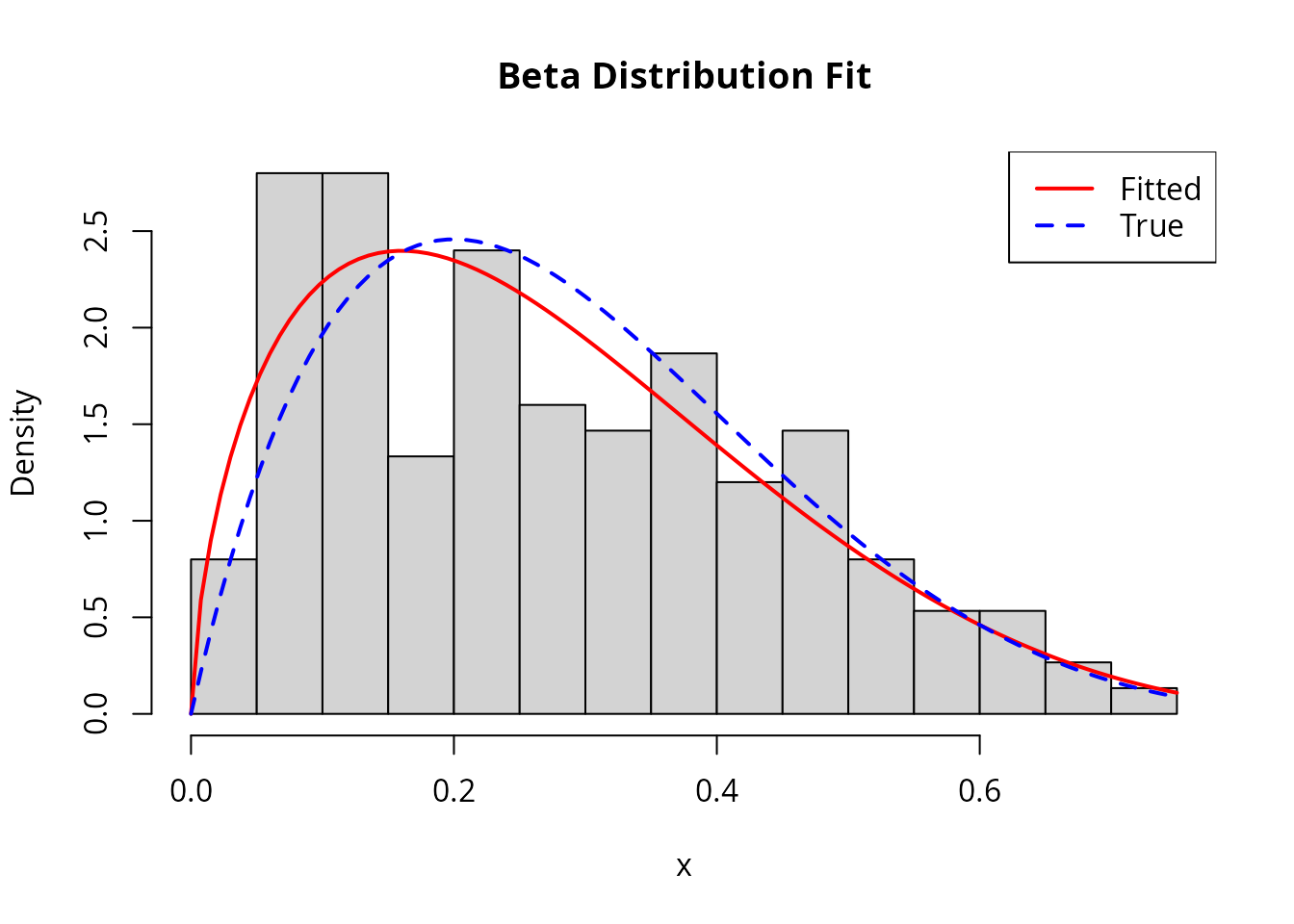

Case Study 4: Weibull Distribution

The Weibull distribution is widely used in reliability analysis and survival modeling. It has shape $k > 0$ and scale $\lambda > 0$ .

Setup

# Generate data
true_k <- 2      # shape
true_lambda <- 3 # scale
x_weibull <- rweibull(100, shape = true_k, scale = true_lambda)

# Log-likelihood
loglike_weibull <- function(theta) {
  k <- theta[1]
  lambda <- theta[2]
  if (k <= 0 || lambda <= 0) return(-Inf)
  n <- length(x_weibull)
  n * log(k) - n * k * log(lambda) +
    (k - 1) * sum(log(x_weibull)) - sum((x_weibull / lambda)^k)
}

# Score function
score_weibull <- function(theta) {
  k <- theta[1]
  lambda <- theta[2]
  n <- length(x_weibull)
  x_scaled <- x_weibull / lambda
  x_scaled_k <- x_scaled^k
  c(
    n / k - n * log(lambda) + sum(log(x_weibull)) - sum(x_scaled_k * log(x_scaled)),
    -n * k / lambda + k * sum(x_scaled_k) / lambda
  )
}

constraint_weibull <- mle_constraint(
  support = function(theta) all(theta > 0),
  project = function(theta) pmax(theta, 1e-6)
)

Fitting with Newton-Raphson

# Fisher information (approximate)
fisher_weibull <- function(theta) {
  k <- theta[1]
  lambda <- theta[2]
  n <- length(x_weibull)
  # Use numerical approximation
  h <- 1e-5
  hess <- matrix(0, 2, 2)
  for (i in 1:2) {
    for (j in 1:2) {
      theta_pp <- theta_pm <- theta_mp <- theta_mm <- theta
      theta_pp[i] <- theta_pp[i] + h
      theta_pp[j] <- theta_pp[j] + h
      theta_pm[i] <- theta_pm[i] + h
      theta_pm[j] <- theta_pm[j] - h
      theta_mp[i] <- theta_mp[i] - h
      theta_mp[j] <- theta_mp[j] + h
      theta_mm[i] <- theta_mm[i] - h
      theta_mm[j] <- theta_mm[j] - h
      hess[i, j] <- (loglike_weibull(theta_pp) - loglike_weibull(theta_pm) -
                     loglike_weibull(theta_mp) + loglike_weibull(theta_mm)) / (4 * h^2)
    }
  }
  -hess
}

result_weibull <- mle_newton_raphson(
  loglike = loglike_weibull,
  score = score_weibull,
  fisher = fisher_weibull,
  theta0 = c(1, 1),
  config = mle_config_linesearch(max_iter = 50),
  constraint = constraint_weibull
)

cat("MLE:  shape =", round(result_weibull$theta.hat[1], 4),
    " scale =", round(result_weibull$theta.hat[2], 4), "\n")
#> MLE:  shape = 2.0469  scale = 2.8593
cat("True: shape =", true_k, " scale =", true_lambda, "\n")
#> True: shape = 2  scale = 3
cat("Iterations:", result_weibull$iter, "\n")
#> Iterations: 10

Visualization

hist(x_weibull, breaks = 15, freq = FALSE, col = "lightgray",
     main = "Weibull Distribution Fit", xlab = "x")
curve(dweibull(x, shape = result_weibull$theta.hat[1],
               scale = result_weibull$theta.hat[2]),
      add = TRUE, col = "red", lwd = 2)
curve(dweibull(x, shape = true_k, scale = true_lambda),
      add = TRUE, col = "blue", lwd = 2, lty = 2)
legend("topright", c("Fitted", "True"), col = c("red", "blue"), lwd = 2, lty = c(1, 2))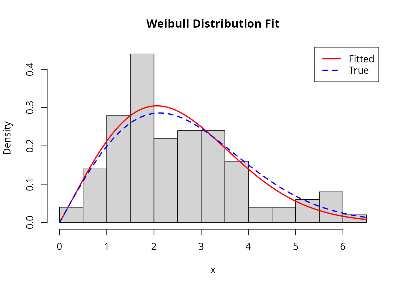

Case Study 5: Mixture of Normals

Mixture models are challenging because the likelihood surface is multimodal. Here we fit a two-component Gaussian mixture.

Setup

# Generate mixture data
n1 <- 60
n2 <- 40
x_mix <- c(rnorm(n1, mean = 0, sd = 1), rnorm(n2, mean = 4, sd = 1.5))

# Parameters: (mu1, sigma1, mu2, sigma2, pi) where pi is mixing proportion
# Log-likelihood for mixture
loglike_mix <- function(theta) {
  mu1 <- theta[1]
  s1 <- theta[2]
  mu2 <- theta[3]
  s2 <- theta[4]
  pi1 <- theta[5]

  if (s1 <= 0 || s2 <= 0 || pi1 <= 0 || pi1 >= 1) return(-Inf)

  # Log-sum-exp trick for numerical stability
  log_p1 <- log(pi1) + dnorm(x_mix, mu1, s1, log = TRUE)
  log_p2 <- log(1 - pi1) + dnorm(x_mix, mu2, s2, log = TRUE)
  log_max <- pmax(log_p1, log_p2)
  sum(log_max + log(exp(log_p1 - log_max) + exp(log_p2 - log_max)))
}

# Numerical score using finite differences
score_mix <- function(theta) {
  h <- 1e-6
  p <- length(theta)
  grad <- numeric(p)
  for (i in 1:p) {
    theta_plus <- theta_minus <- theta
    theta_plus[i] <- theta_plus[i] + h
    theta_minus[i] <- theta_minus[i] - h
    grad[i] <- (loglike_mix(theta_plus) - loglike_mix(theta_minus)) / (2 * h)
  }
  grad
}

constraint_mix <- mle_constraint(
  support = function(theta) {
    theta[2] > 0 && theta[4] > 0 && theta[5] > 0 && theta[5] < 1
  },
  project = function(theta) {
    c(theta[1], max(theta[2], 0.1), theta[3], max(theta[4], 0.1),
      min(max(theta[5], 0.01), 0.99))
  }
)

Fitting with Good Starting Values

# Use k-means to get good starting values
km <- kmeans(x_mix, centers = 2)
mu1_init <- min(km$centers)
mu2_init <- max(km$centers)
s1_init <- sd(x_mix[km$cluster == which.min(km$centers)])
s2_init <- sd(x_mix[km$cluster == which.max(km$centers)])
pi_init <- mean(km$cluster == which.min(km$centers))

# Fit from the k-means initialization
result_mix <- mle_gradient_ascent(
  loglike = loglike_mix,
  score = score_mix,
  theta0 = c(mu1_init, s1_init, mu2_init, s2_init, pi_init),
  config = mle_config_linesearch(max_iter = 300, max_step = 0.5),
  constraint = constraint_mix
)

cat("Fitted mixture parameters:\n")
#> Fitted mixture parameters:
cat("  Component 1: mu =", round(result_mix$theta.hat[1], 2),
    " sigma =", round(result_mix$theta.hat[2], 2), "\n")
#>   Component 1: mu = -0.07  sigma = 0.93
cat("  Component 2: mu =", round(result_mix$theta.hat[3], 2),
    " sigma =", round(result_mix$theta.hat[4], 2), "\n")
#>   Component 2: mu = 4.38  sigma = 1.37
cat("  Mixing proportion:", round(result_mix$theta.hat[5], 2), "\n")
#>   Mixing proportion: 0.59
cat("\nTrue parameters:\n")
#> 
#> True parameters:
cat("  Component 1: mu = 0, sigma = 1\n")
#>   Component 1: mu = 0, sigma = 1
cat("  Component 2: mu = 4, sigma = 1.5\n")
#>   Component 2: mu = 4, sigma = 1.5
cat("  Mixing proportion:", n1 / (n1 + n2), "\n")
#>   Mixing proportion: 0.6

Visualization

hist(x_mix, breaks = 25, freq = FALSE, col = "lightgray",
     main = "Gaussian Mixture Fit", xlab = "x")

# Fitted density
x_seq <- seq(min(x_mix) - 1, max(x_mix) + 1, length.out = 200)
fitted_density <- result_mix$theta.hat[5] *
  dnorm(x_seq, result_mix$theta.hat[1], result_mix$theta.hat[2]) +
  (1 - result_mix$theta.hat[5]) *
  dnorm(x_seq, result_mix$theta.hat[3], result_mix$theta.hat[4])
lines(x_seq, fitted_density, col = "red", lwd = 2)

# True density
true_density <- (n1/(n1+n2)) * dnorm(x_seq, 0, 1) +
  (n2/(n1+n2)) * dnorm(x_seq, 4, 1.5)
lines(x_seq, true_density, col = "blue", lwd = 2, lty = 2)

legend("topright", c("Fitted", "True"), col = c("red", "blue"), lwd = 2, lty = c(1, 2))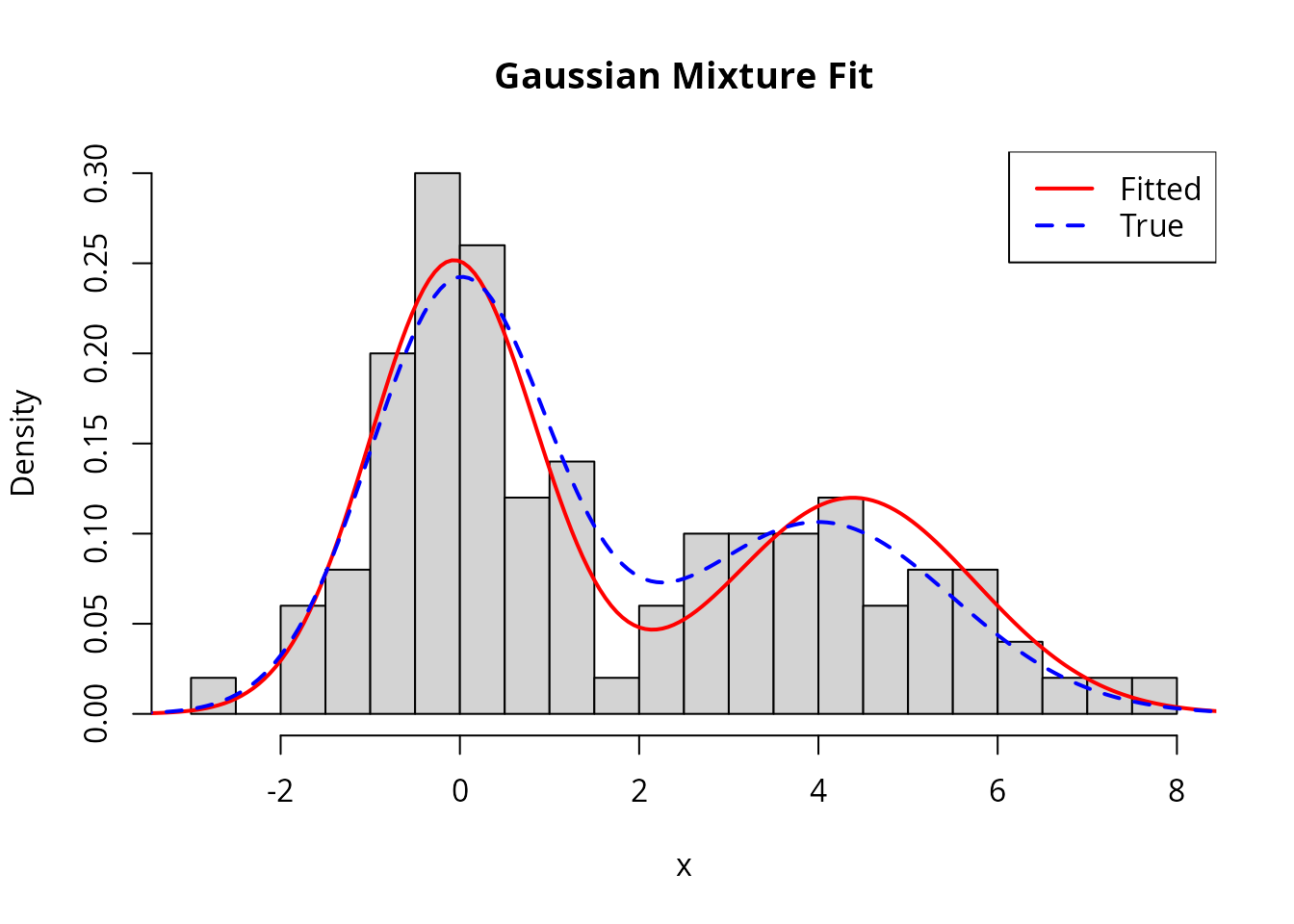

Case Study 6: Logistic Regression

Logistic regression models binary outcomes. This demonstrates MLE for a generalized linear model.

Setup

# Generate data
n <- 200
x1 <- rnorm(n)
x2 <- rnorm(n)
true_beta <- c(0.5, 1.5, -1)  # intercept, beta1, beta2
eta <- true_beta[1] + true_beta[2] * x1 + true_beta[3] * x2
prob <- 1 / (1 + exp(-eta))
y <- rbinom(n, 1, prob)

# Log-likelihood
loglike_logistic <- function(beta) {
  eta <- beta[1] + beta[2] * x1 + beta[3] * x2
  sum(y * eta - log(1 + exp(eta)))
}

# Score function
score_logistic <- function(beta) {
  eta <- beta[1] + beta[2] * x1 + beta[3] * x2
  p <- 1 / (1 + exp(-eta))
  resid <- y - p
  c(sum(resid), sum(resid * x1), sum(resid * x2))
}

# Fisher information
fisher_logistic <- function(beta) {
  eta <- beta[1] + beta[2] * x1 + beta[3] * x2
  p <- 1 / (1 + exp(-eta))
  w <- p * (1 - p)
  X <- cbind(1, x1, x2)
  t(X) %*% diag(w) %*% X
}

Fitting

result_logistic <- mle_newton_raphson(
  loglike = loglike_logistic,
  score = score_logistic,
  fisher = fisher_logistic,
  theta0 = c(0, 0, 0),
  config = mle_config_linesearch(max_iter = 50)
)

# Compare with glm
glm_fit <- glm(y ~ x1 + x2, family = binomial)

cat("Newton-Raphson MLE:\n")
#> Newton-Raphson MLE:
cat("  ", round(result_logistic$theta.hat, 4), "\n")
#>    0.6478 1.544 -1.1066
cat("GLM estimates:\n")
#> GLM estimates:
cat("  ", round(coef(glm_fit), 4), "\n")
#>    0.6475 1.5439 -1.1067
cat("True parameters:\n")
#> True parameters:
cat("  ", true_beta, "\n")
#>    0.5 1.5 -1
cat("\nIterations:", result_logistic$iter, "\n")
#> 
#> Iterations: 4

Case Study 7: Poisson Regression with Regularization

This demonstrates penalized MLE for count data with many predictors.

Setup

# Generate data with some irrelevant predictors
n <- 150
p <- 10
X <- matrix(rnorm(n * p), n, p)
true_beta <- c(0.5, 0.3, -0.4, rep(0, p - 3))  # Only first 3 are relevant
lambda <- exp(X %*% true_beta)
y_pois <- rpois(n, lambda)

# Log-likelihood
loglike_pois <- function(beta) {
  eta <- X %*% beta
  sum(y_pois * eta - exp(eta))
}

# Score
score_pois <- function(beta) {
  eta <- X %*% beta
  resid <- y_pois - exp(eta)
  as.vector(t(X) %*% resid)
}

Fitting with L2 Regularization

# Add L2 penalty for shrinkage (ridge regression)
loglike_pois_l2 <- with_penalty(loglike_pois, penalty_l2(), lambda = 0.1)

# Score for L2 penalized likelihood
score_pois_l2 <- function(beta) {
  eta <- X %*% beta
  resid <- y_pois - exp(eta)
  as.vector(t(X) %*% resid) - 0.2 * beta  # gradient of L2 penalty
}

result_pois <- mle_gradient_ascent(
  loglike = loglike_pois_l2,
  score = score_pois_l2,
  theta0 = rep(0, p),
  config = mle_config_linesearch(max_iter = 200, max_step = 0.5)
)

cat("Estimated coefficients (L2 regularized):\n")
#> Estimated coefficients (L2 regularized):
print(round(result_pois$theta.hat, 3))
#>  [1]  0.520  0.240 -0.463  0.033  0.097 -0.014 -0.121 -0.011 -0.009 -0.062
cat("\nTrue coefficients:\n")
#> 
#> True coefficients:
print(round(true_beta, 3))
#>  [1]  0.5  0.3 -0.4  0.0  0.0  0.0  0.0  0.0  0.0  0.0

Summary

This vignette demonstrated numerical.mle across various statistical models:

Distribution	Parameters	Challenges	Recommended Approach
Exponential	1	Simple	Gradient ascent
Gamma	2	Digamma function	Line search
Beta	2	Bounded data	Good initialization
Weibull	2	Nonlinear	Newton-Raphson
Mixture	5+	Multimodal	K-means initialization
Logistic	p	GLM structure	Newton-Raphson
Poisson (reg)	p	Many parameters	Regularization

Key takeaways:

Always use constraints to keep parameters in valid ranges
Try multiple starting points for complex likelihoods
Newton-Raphson converges faster when Fisher information is available
Use regularization when you have many parameters
Visualize the likelihood surface for 1-2 parameter problems

Alexander Towell

2025-12-02

Introduction

Case Study 1: Exponential Distribution

Setup

Fitting

Visualization

Case Study 2: Gamma Distribution

Setup

Fitting with Different Methods

Visualization

Case Study 3: Beta Distribution

Setup

Fitting

Checking the Fit

Case Study 4: Weibull Distribution

Setup

Fitting with Newton-Raphson

Visualization

Case Study 5: Mixture of Normals

Setup

Fitting with Good Starting Values

Visualization

Case Study 6: Logistic Regression

Setup

Fitting

Case Study 7: Poisson Regression with Regularization

Setup

Fitting with L2 Regularization

Summary