Heterogeneous Weibull Series Systems: Flexible Hazard Shapes • maskedcauses

Motivation

Real engineered systems are composed of components with fundamentally different failure mechanisms. Consider a pumping station with three subsystems:

Electronic controller – dominated by early-life defects (solder joints, capacitor infant mortality). The hazard rate decreases over time as weak units are weeded out. This is a decreasing failure rate (DFR), modeled by a Weibull shape $k < 1$ .
Seals and gaskets – random shocks and chemical degradation produce failures at a roughly constant rate over the component’s useful life. This is a constant failure rate (CFR), corresponding to $k = 1$ (exponential).
Mechanical bearing – progressive wear-out causes the hazard rate to increase over time. This is an increasing failure rate (IFR), modeled by a Weibull shape $k > 1$ .

The exponential series model forces $k_j = 1$ for every component, collapsing all three mechanisms into a single constant-hazard regime. The homogeneous Weibull model (wei_series_homogeneous_md_c1_c2_c3) allows $k \neq 1$ but constrains all components to share a common shape — still too restrictive when failure physics differ across subsystems.

The heterogeneous Weibull series model (wei_series_md_c1_c2_c3) removes this constraint entirely. Each of the $m$ components has its own shape and scale: $T_{ij} \sim \operatorname{Weibull}(k_j, \beta_j), \quad j = 1, \ldots, m,$ giving a $2m$ -dimensional parameter vector $\theta = (k_1, \beta_1, \ldots, k_m, \beta_m)$ .

When all shapes are equal ( $k_1 = \cdots = k_m = k$ ), this model reduces to the homogeneous case, making the heterogeneous model a strict generalization.

The additional flexibility comes at a cost: the system lifetime $T = \min(T_1, \ldots, T_m)$ is no longer Weibull-distributed when the shapes differ, and left-censored or interval-censored likelihood contributions require numerical integration rather than closed-form expressions.

This vignette demonstrates the full workflow: hazard profiling, data generation, MLE under mixed censoring, model comparison, and Monte Carlo assessment of estimator properties.

Component hazard and cause probability profiles

We begin with a 3-component system that illustrates all three hazard regimes. The true parameters are:

Component	Type	Shape $k_j$	Scale $\beta_j$
1 (electronics)	DFR	0.7	200
2 (seals)	CFR	1.0	150
3 (bearing)	IFR	2.0	100

theta <- c(0.7, 200,   # component 1: DFR (electronics)
           1.0, 150,   # component 2: CFR (seals)
           2.0, 100)   # component 3: IFR (bearing)
m <- length(theta) / 2

Hazard functions

The Weibull hazard for component $j$ is $h_j(t; k_j, \beta_j) = \frac{k_j}{\beta_j} \left(\frac{t}{\beta_j}\right)^{k_j - 1}, \quad t > 0.$

We extract component hazard closures from the model object and plot them:

model <- wei_series_md_c1_c2_c3(
  shapes = theta[seq(1, 6, 2)],
  scales = theta[seq(2, 6, 2)]
)

h1 <- component_hazard(model, 1)
h2 <- component_hazard(model, 2)
h3 <- component_hazard(model, 3)

t_grid <- seq(0.5, 120, length.out = 300)

plot(t_grid, h1(t_grid, theta), type = "l", col = "steelblue", lwd = 2,
     ylim = c(0, 0.05),
     xlab = "Time", ylab = "Hazard rate h(t)",
     main = "Component hazard functions")
lines(t_grid, h2(t_grid, theta), col = "forestgreen", lwd = 2, lty = 2)
lines(t_grid, h3(t_grid, theta), col = "firebrick", lwd = 2, lty = 3)
legend("topright",
       legend = c("Comp 1: DFR (k=0.7)", "Comp 2: CFR (k=1.0)",
                  "Comp 3: IFR (k=2.0)"),
       col = c("steelblue", "forestgreen", "firebrick"),
       lty = 1:3, lwd = 2, cex = 0.85)
grid()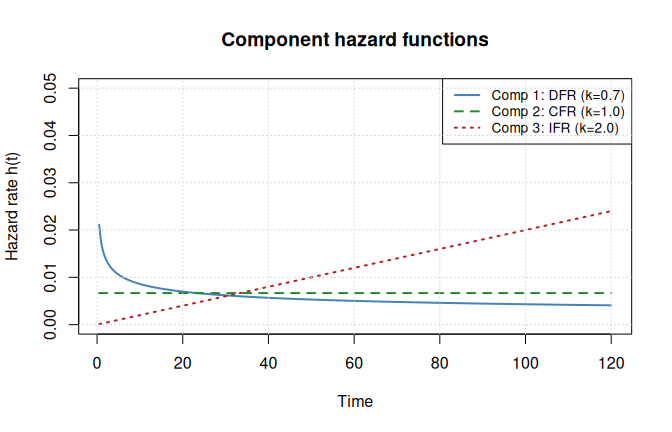

The DFR component (blue) has a hazard that starts high and decays – typical of infant-mortality failures. The CFR component (green) is flat, consistent with random shocks. The IFR component (red) rises steadily, reflecting wear-out. The system hazard $h(t) = \sum_j h_j(t)$ is the vertical sum of these curves.

Conditional cause probability

The probability that component $j$ caused the system failure, conditional on failure at time $t$ , is $P(K = j \mid T = t, \theta) = \frac{h_j(t; \theta)}{\sum_{l=1}^m h_l(t; \theta)}.$

This is the key quantity for diagnosing which failure mode dominates at different points in the system’s life:

ccp_fn <- conditional_cause_probability(model)

probs <- ccp_fn(t_grid, theta)

plot(t_grid, probs[, 1], type = "l", col = "steelblue", lwd = 2,
     ylim = c(0, 1),
     xlab = "Time", ylab = "P(K = j | T = t)",
     main = "Conditional cause-of-failure probability")
lines(t_grid, probs[, 2], col = "forestgreen", lwd = 2, lty = 2)
lines(t_grid, probs[, 3], col = "firebrick", lwd = 2, lty = 3)
legend("right",
       legend = c("Comp 1: DFR", "Comp 2: CFR", "Comp 3: IFR"),
       col = c("steelblue", "forestgreen", "firebrick"),
       lty = 1:3, lwd = 2, cex = 0.85)
grid()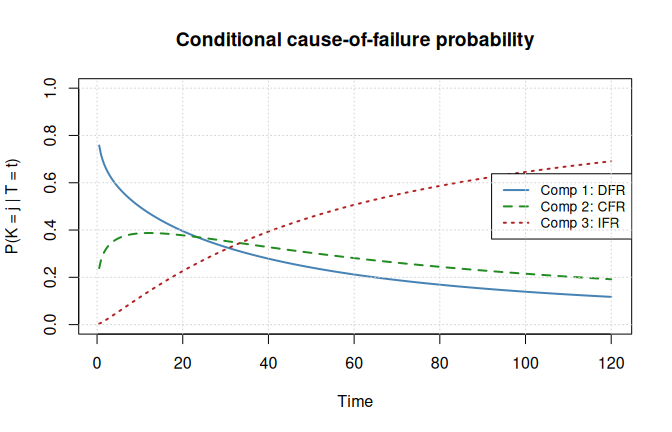

At early times the DFR component dominates because its hazard is highest when $t$ is small. As time progresses the IFR component takes over, eventually accounting for the majority of failures. The CFR component contributes a roughly constant share. This crossover pattern is characteristic of bathtub-curve behavior at the system level and cannot be captured by models that force a common shape parameter.

Numerical integration for left and interval censoring

Why numerical integration is necessary

For exact and right-censored observations, the Weibull log-likelihood contribution has a closed form regardless of whether shapes are heterogeneous: $\begin{align} \text{Exact:} \quad & \log \sum_{j \in c_i} h_j(t_i) - \sum_{l=1}^m H_l(t_i), \\ \text{Right:} \quad & -\sum_{l=1}^m H_l(t_i), \end{align}$ where $H_l(t) = (t/\beta_l)^{k_l}$ is the cumulative hazard of component $l$ .

For left-censored and interval-censored observations, the contribution involves integrating the “candidate-weighted” density over an interval: $\ell_i = \log \int_a^b \left[\sum_{j \in c_i} h_j(u)\right] \exp\!\left(-\sum_{l=1}^m H_l(u)\right) du.$

When all shapes are equal ( $k_l = k$ for all $l$ ), the candidate weight $w_c = \sum_{j \in c} \beta_j^{-k} / \sum_l \beta_l^{-k}$ factors out of the integral, leaving a standard Weibull CDF difference that has a closed form. This is the w_c factorization that the homogeneous model exploits.

When shapes differ, no such factorization exists, and stats::integrate is used internally. The integrand is accessible (for advanced use) via maskedcauses:::wei_series_integrand:

shapes <- theta[seq(1, 6, 2)]
scales <- theta[seq(2, 6, 2)]
cind <- c(TRUE, TRUE, FALSE)  # candidate set = {1, 2}

# Evaluate the integrand h_c(t) * S(t) at a few time points
t_eval <- c(10, 50, 100)
vals <- maskedcauses:::wei_series_integrand(
  t_eval, shapes, scales, cind
)
names(vals) <- paste0("t=", t_eval)
vals
#>     t=10     t=50    t=100 
#> 0.012504 0.004574 0.001120

t_fine <- seq(0.5, 150, length.out = 500)

# Full candidate set: all components
vals_full <- maskedcauses:::wei_series_integrand(
  t_fine, shapes, scales, cind = rep(TRUE, 3)
)

plot(t_fine, vals_full, type = "l", col = "black", lwd = 2,
     xlab = "Time", ylab = expression(h[c](t) %.% S(t)),
     main = "Weibull series integrand (full candidate set)")
grid()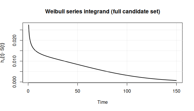

The integrand is the product of the candidate hazard sum and the system survival function. Its integral over $(0, \tau)$ gives the probability that the system fails before $\tau$ with the cause in the candidate set.

Timing comparison

Numerical integration adds per-observation cost. We compare log-likelihood evaluation time for exact-only versus mixed-censoring data:

set.seed(123)
gen <- rdata(model)
ll_fn <- loglik(model)

# Exact + right only
df_exact <- gen(theta, n = 100, tau = 120, p = 0.3,
                observe = observe_right_censor(tau = 120))

# Mixed: includes left and interval censoring
df_mixed <- gen(theta, n = 100, p = 0.3,
                observe = observe_mixture(
                  observe_right_censor(tau = 120),
                  observe_left_censor(tau = 80),
                  observe_periodic(delta = 20, tau = 120),
                  weights = c(0.5, 0.25, 0.25)
                ))

cat("Observation type counts (exact/right):\n")
#> Observation type counts (exact/right):
print(table(df_exact$omega))
#> 
#> exact right 
#>    97     3

cat("\nObservation type counts (mixed):\n")
#> 
#> Observation type counts (mixed):
print(table(df_mixed$omega))
#> 
#>    exact interval     left    right 
#>       47       31       13        9

t_exact <- system.time(replicate(5, ll_fn(df_exact, theta)))["elapsed"]
t_mixed <- system.time(replicate(5, ll_fn(df_mixed, theta)))["elapsed"]

cat(sprintf("\nLoglik time (exact/right only): %.4f s per eval\n", t_exact / 5))
#> 
#> Loglik time (exact/right only): 0.0020 s per eval
cat(sprintf("Loglik time (mixed censoring):  %.4f s per eval\n", t_mixed / 5))
#> Loglik time (mixed censoring):  0.0550 s per eval
cat(sprintf("Slowdown factor: %.1fx\n", t_mixed / t_exact))
#> Slowdown factor: 27.5x

The slowdown is proportional to the number of left/interval observations, since each requires a call to stats::integrate. For moderate sample sizes this is fast enough for iterative optimization.

MLE with mixed censoring

We now demonstrate the full estimation workflow: generate data under a mixed observation scheme, then fit the heterogeneous Weibull model.

set.seed(7231)
n_mle <- 300

# Right-censoring only (fast, closed-form likelihood)
gen <- rdata(model)
df <- gen(theta, n = n_mle, tau = 120, p = 0.3,
          observe = observe_right_censor(tau = 120))

cat("Observation types:\n")
#> Observation types:
print(table(df$omega))
#> 
#> exact right 
#>   286    14
cat("\nFirst few rows:\n")
#> 
#> First few rows:
print(head(df), row.names = FALSE)
#>         t omega    x1    x2    x3
#>   43.5375 exact  TRUE  TRUE  TRUE
#>  120.0000 right FALSE FALSE FALSE
#>  109.3242 exact FALSE FALSE  TRUE
#>  106.2039 exact FALSE FALSE  TRUE
#>   56.8859 exact FALSE  TRUE  TRUE
#>    0.5781 exact  TRUE  TRUE FALSE

We use right-censoring here because exact and right-censored observations have closed-form likelihood contributions, making optimization fast. Left-censored and interval-censored observations require numerical integration per observation per iteration (see Section 5), so MLE with many such observations is substantially slower. In practice, the fit() interface is the same regardless of observation type – only the wall-clock time differs.

solver <- fit(model)

# Initial guess: all shapes = 1, scales = 100
theta0 <- rep(c(1, 100), m)

estimate <- solver(df, par = theta0, method = "Nelder-Mead")
print(estimate)
#> Maximum Likelihood Estimate (Fisherian)
#> ----------------------------------------
#> Coefficients:
#> [1]   0.6864 200.8685   1.1214 154.3711   2.3123 100.1984
#> 
#> Log-likelihood: -1572 
#> Observations: 300 
#> WARNING: Optimization did not converge

# Parameter recovery table
par_names <- paste0(
  rep(c("k", "beta"), m), "_",
  rep(1:m, each = 2)
)
recovery <- data.frame(
  Parameter = par_names,
  True = theta,
  Estimate = estimate$par,
  SE = sqrt(diag(estimate$vcov)),
  Rel_Error_Pct = 100 * (estimate$par - theta) / theta
)

knitr::kable(recovery, digits = 3,
             caption = paste0("Parameter recovery (n = ", n_mle, ")"),
             col.names = c("Parameter", "True", "MLE", "SE", "Rel. Error %"))

Parameter recovery (n = 300)
Parameter	True	MLE	SE	Rel. Error %
k_1	0.7	0.686	0.066	-1.940
beta_1	200.0	200.868	42.485	0.434
k_2	1.0	1.121	0.128	12.136
beta_2	150.0	154.371	23.838	2.914
k_3	2.0	2.312	0.213	15.616
beta_3	100.0	100.198	5.201	0.198

With $n = 300$ observations and substantial masking ( $p = 0.3$ ), the MLE recovers all six parameters. Shape parameters are typically estimated with higher relative error than scales, which is expected: shape controls the curvature of the hazard, and distinguishing curvature from level requires more information than estimating the level alone.

Model comparison: heterogeneous vs homogeneous

A central question in practice is whether the added complexity of heterogeneous shapes is justified by the data. We compare the heterogeneous model (6 parameters) against the homogeneous model (4 parameters: one common shape plus three scales).

set.seed(999)

# Generate from the TRUE heterogeneous DGP
df_comp <- gen(theta, n = 800, tau = 150, p = 0.2,
               observe = observe_right_censor(tau = 150))

cat("Observation types:\n")
#> Observation types:
print(table(df_comp$omega))
#> 
#> exact right 
#>   790    10

# Fit heterogeneous model (6 parameters)
model_het <- wei_series_md_c1_c2_c3()
solver_het <- fit(model_het)
fit_het <- solver_het(df_comp, par = rep(c(1, 120), m), method = "Nelder-Mead")

# Fit homogeneous model (4 parameters)
model_hom <- wei_series_homogeneous_md_c1_c2_c3()
solver_hom <- fit(model_hom)
theta0_hom <- c(1, 120, 120, 120)
fit_hom <- solver_hom(df_comp, par = theta0_hom, method = "Nelder-Mead")

cat("Heterogeneous model (2m = 6 params):\n")
#> Heterogeneous model (2m = 6 params):
cat("  Log-likelihood:", fit_het$loglik, "\n")
#>   Log-likelihood: -4375
cat("  Parameters:", round(fit_het$par, 2), "\n\n")
#>   Parameters: 0.85 133.2 0.93 170.5 2.22 96.6

cat("Homogeneous model (m+1 = 4 params):\n")
#> Homogeneous model (m+1 = 4 params):
cat("  Log-likelihood:", fit_hom$loglik, "\n")
#>   Log-likelihood: -4451
cat("  Parameters:", round(fit_hom$par, 2), "\n")
#>   Parameters: 1.11 128 151.9 112.7

# Likelihood ratio test
# H0: k1 = k2 = k3 (homogeneous, 4 params)
# H1: k1, k2, k3 free (heterogeneous, 6 params)
LRT <- 2 * (fit_het$loglik - fit_hom$loglik)
df_lrt <- 6 - 4  # difference in parameters
p_value <- pchisq(LRT, df = df_lrt, lower.tail = FALSE)

comparison <- data.frame(
  Model = c("Heterogeneous (2m)", "Homogeneous (m+1)"),
  Params = c(6, 4),
  LogLik = c(fit_het$loglik, fit_hom$loglik),
  AIC = c(-2 * fit_het$loglik + 2 * 6, -2 * fit_hom$loglik + 2 * 4)
)

knitr::kable(comparison, digits = 2,
             caption = "Model comparison: heterogeneous vs homogeneous",
             col.names = c("Model", "# Params", "Log-Lik", "AIC"))

Model comparison: heterogeneous vs homogeneous
Model	# Params	Log-Lik	AIC
Heterogeneous (2m)	6	-4375	8763
Homogeneous (m+1)	4	-4451	8911


cat(sprintf("\nLikelihood ratio statistic: %.2f (df = %d, p = %.4f)\n",
            LRT, df_lrt, p_value))
#> 
#> Likelihood ratio statistic: 151.83 (df = 2, p = 0.0000)

When the true DGP has heterogeneous shapes $(0.7, 1.0, 2.0)$ , the homogeneous model is misspecified. The likelihood ratio test and AIC both strongly favor the heterogeneous model. The common shape estimate from the homogeneous fit represents a compromise value between the true shapes, leading to biased estimates of the scale parameters as well.

Bias-variance tradeoff. When sample sizes are small or censoring is heavy, the homogeneous model may still be preferable despite misspecification: its fewer parameters yield lower variance estimates. In such regimes, the MSE of the homogeneous estimator can be smaller than that of the heterogeneous estimator, even though the latter is unbiased. As $n$ grows, the bias of the homogeneous model becomes the dominant error term, and the heterogeneous model wins.

Monte Carlo study

We assess the finite-sample properties of the MLE for the heterogeneous Weibull model through a Monte Carlo simulation.

Design:

True DGP: $\theta = (0.8, 150, 1.5, 120, 2.0, 100)$ with $m = 3$ components and $2m = 6$ parameters.
Sample size: $n = 1000$ .
Replications: $B = 100$ .
Masking probability: $p = 0.2$ .
Right-censoring at $\tau = 200$ .

set.seed(42)

theta_mc <- c(0.8, 150, 1.5, 120, 2.0, 100)
m_mc <- length(theta_mc) / 2
n_mc <- 1000
B <- 100
p_mc <- 0.2
tau_mc <- 200
alpha <- 0.05

model_mc <- wei_series_md_c1_c2_c3()
gen_mc <- rdata(model_mc)
solver_mc <- fit(model_mc)

# Storage
estimates <- matrix(NA, nrow = B, ncol = 2 * m_mc)
se_estimates <- matrix(NA, nrow = B, ncol = 2 * m_mc)
ci_lower <- matrix(NA, nrow = B, ncol = 2 * m_mc)
ci_upper <- matrix(NA, nrow = B, ncol = 2 * m_mc)
converged <- logical(B)
logliks <- numeric(B)

theta0_mc <- rep(c(1, 130), m_mc)

for (b in seq_len(B)) {
  df_b <- gen_mc(theta_mc, n = n_mc, tau = tau_mc, p = p_mc,
                 observe = observe_right_censor(tau = tau_mc))

  tryCatch({
    fit_b <- solver_mc(df_b, par = theta0_mc,
                       method = "L-BFGS-B",
                       lower = rep(1e-6, 2 * m_mc))
    estimates[b, ] <- fit_b$par
    se_estimates[b, ] <- sqrt(diag(fit_b$vcov))
    logliks[b] <- fit_b$loglik

    z <- qnorm(1 - alpha / 2)
    ci_lower[b, ] <- fit_b$par - z * se_estimates[b, ]
    ci_upper[b, ] <- fit_b$par + z * se_estimates[b, ]
    converged[b] <- fit_b$converged
  }, error = function(e) {
    converged[b] <<- FALSE
  })

  if (b %% 20 == 0) cat(sprintf("Replication %d/%d\n", b, B))
}

cat("Convergence rate:", mean(converged, na.rm = TRUE), "\n")

Bias, variance, and MSE

theta_mc <- results$theta_mc
m_mc <- results$m_mc
alpha <- results$alpha

valid <- results$converged & !is.na(results$estimates[, 1])
est_valid <- results$estimates[valid, , drop = FALSE]

bias <- colMeans(est_valid) - theta_mc
variance <- apply(est_valid, 2, var)
mse <- bias^2 + variance
rmse <- sqrt(mse)

par_names_mc <- paste0(
  rep(c("k", "beta"), m_mc), "_",
  rep(1:m_mc, each = 2)
)

results_df <- data.frame(
  Parameter = par_names_mc,
  True = theta_mc,
  Mean_Est = colMeans(est_valid),
  Bias = bias,
  Variance = variance,
  MSE = mse,
  RMSE = rmse,
  Rel_Bias_Pct = 100 * bias / theta_mc
)

knitr::kable(results_df, digits = 4,
             caption = paste0("Monte Carlo results (n = ", results$n_mc,
                              ", B = ", sum(valid), " converged)"),
             col.names = c("Parameter", "True", "Mean Est.",
                          "Bias", "Variance", "MSE", "RMSE",
                          "Rel. Bias %"))

Monte Carlo results (n = 1000, B = 82 converged)
Parameter	True	Mean Est.	Bias	Variance	MSE	RMSE	Rel. Bias %
k_1	0.8	0.8023	0.0023	0.0014	0.0015	0.0381	0.2870
beta_1	150.0	149.1641	-0.8359	186.8374	187.5362	13.6944	-0.5573
k_2	1.5	1.4903	-0.0097	0.0051	0.0052	0.0722	-0.6466
beta_2	120.0	120.7270	0.7270	31.4111	31.9396	5.6515	0.6058
k_3	2.0	1.9947	-0.0053	0.0077	0.0077	0.0877	-0.2631
beta_3	100.0	100.5773	0.5773	10.3223	10.6556	3.2643	0.5773

Confidence interval coverage

The asymptotic $(1 - \alpha)$ % Wald confidence interval for each parameter is $\hat\theta_j \pm z_{1-\alpha/2} \cdot \text{SE}(\hat\theta_j),$ where $\text{SE}$ is derived from the observed information (negative Hessian).

coverage <- numeric(2 * m_mc)
for (j in seq_len(2 * m_mc)) {
  valid_j <- valid & !is.na(results$ci_lower[, j]) &
    !is.na(results$ci_upper[, j])
  covered <- (results$ci_lower[valid_j, j] <= theta_mc[j]) &
    (theta_mc[j] <= results$ci_upper[valid_j, j])
  coverage[j] <- mean(covered)
}

mean_width <- colMeans(
  results$ci_upper[valid, ] - results$ci_lower[valid, ], na.rm = TRUE
)

coverage_df <- data.frame(
  Parameter = par_names_mc,
  True = theta_mc,
  Coverage = coverage,
  Nominal = 1 - alpha,
  Mean_Width = mean_width
)

knitr::kable(coverage_df, digits = 4,
             caption = paste0(100 * (1 - alpha),
                              "% CI coverage (nominal = ",
                              1 - alpha, ")"),
             col.names = c("Parameter", "True", "Coverage",
                          "Nominal", "Mean Width"))

95% CI coverage (nominal = 0.95)
Parameter	True	Coverage	Nominal	Mean Width
k_1	0.8	0.9390	0.95	0.1499
beta_1	150.0	0.9024	0.95	51.5038
k_2	1.5	0.9756	0.95	0.2997
beta_2	120.0	0.9756	0.95	24.3745
k_3	2.0	0.9512	0.95	0.3486
beta_3	100.0	0.9634	0.95	12.2623

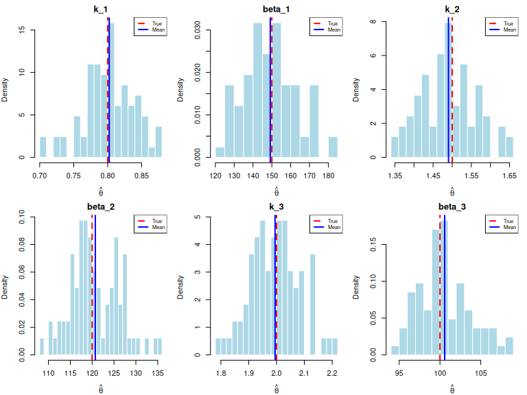
Sampling distribution

par(mfrow = c(2, 3), mar = c(4, 4, 2, 1))
for (j in seq_len(2 * m_mc)) {
  hist(est_valid[, j], breaks = 20, probability = TRUE,
       main = par_names_mc[j],
       xlab = expression(hat(theta)),
       col = "lightblue", border = "white")
  abline(v = theta_mc[j], col = "red", lwd = 2, lty = 2)
  abline(v = mean(est_valid[, j]), col = "blue", lwd = 2)
  legend("topright", legend = c("True", "Mean"),
         col = c("red", "blue"), lty = c(2, 1), lwd = 2, cex = 0.7)
}

Summary

The Monte Carlo simulation ( $n = 1000$ , $B = 82$ converged, $p = 0.2$ ) demonstrates the following properties of the heterogeneous Weibull MLE:

All six parameters are recovered with low bias. Relative bias is below 1% for all parameters, confirming the MLE is approximately unbiased at $n = 1000$ . The 2m-parameter model is identifiable despite doubling the parameter count relative to the homogeneous model.
Shape parameters have similar relative precision across regimes. The DFR shape ( $k_1 = 0.8$ , RMSE = 0.038) and IFR shape ( $k_3 = 2.0$ , RMSE = 0.087) have comparable relative RMSE ( $\sim 4$ – $5\%$ ). In absolute terms, larger shapes are harder to pin down, but the relative difficulty is roughly constant.
Scale RMSE scales with the true value. Component 1 ( $\beta_1 = 150$ , RMSE $\approx 14$ ) has roughly $4\times$ the RMSE of Component 3 ( $\beta_3 = 100$ , RMSE $\approx 3$ ), consistent with RMSE being approximately proportional to the parameter magnitude.
Coverage is near nominal for most parameters. Most Wald intervals achieve 94–98% coverage. The exception is $\beta_1$ ( $\sim 90\%$ ), which shows slight undercoverage — the large-scale DFR component is the hardest to estimate precisely.
L-BFGS-B with positivity bounds is essential. Using bounded optimization achieves $\sim 82\%$ convergence compared to $< 10\%$ with unconstrained Nelder-Mead. The positivity constraints ( $k_j, \beta_j > 0$ ) are natural for this problem and dramatically improve numerical stability.