Homogeneous Weibull Series Systems: Shared Shape Parameter

Theory

Component lifetime model

Consider a series system with $m$ components where each component lifetime follows a Weibull distribution with a common shape parameter $k$ but individual scale parameters $\beta_1, \ldots, \beta_m$. The parameter vector is $$\theta = (k, \beta_1, \ldots, \beta_m) \in \mathbb{R}^{m+1}_{>0}.$$

The $j$-th component has hazard function $$h_j(t \mid k, \beta_j) = \frac{k}{\beta_j} \left(\frac{t}{\beta_j}\right)^{k-1}, \quad t > 0,$$ survival function $$R_j(t \mid k, \beta_j) = \exp\!\left(-\left(\frac{t}{\beta_j}\right)^k\right),$$ and pdf $$f_j(t \mid k, \beta_j) = h_j(t) \, R_j(t) = \frac{k}{\beta_j}\left(\frac{t}{\beta_j}\right)^{k-1} \exp\!\left(-\left(\frac{t}{\beta_j}\right)^k\right).$$

The shape parameter $k$ controls the failure rate behaviour:

• $k < 1$: decreasing failure rate (DFR) – infant mortality, burn-in
• $k = 1$: constant failure rate (CFR) – exponential distribution
• $k > 1$: increasing failure rate (IFR) – wear-out, aging

System lifetime

The system lifetime $T = \min(T_1, \ldots, T_m)$ has reliability $$R_{\text{sys}}(t \mid \theta) = \prod_{j=1}^m R_j(t) = \exp\!\left(-\sum_{j=1}^m \left(\frac{t}{\beta_j}\right)^k\right).$$

Because all components share the same shape $k$, the exponent simplifies: $$\sum_{j=1}^m \left(\frac{t}{\beta_j}\right)^k = t^k \sum_{j=1}^m \beta_j^{-k} = \left(\frac{t}{\beta_{\text{sys}}}\right)^k,$$ where $$\beta_{\text{sys}} = \left(\sum_{j=1}^m \beta_j^{-k}\right)^{-1/k}.$$ Thus, the system lifetime is itself Weibull with shape $k$ and scale $\beta_{\text{sys}}$: $$T \sim \operatorname{Weibull}(k, \beta_{\text{sys}}).$$ This closure under the minimum operation is the defining structural advantage of the homogeneous model and is computed by wei_series_system_scale(k, scales).

Conditional cause probability

The conditional probability that component $j$ caused the system failure at time $t$ is $$P(K = j \mid T = t, \theta) = \frac{h_j(t)}{h_{\text{sys}}(t)} = \frac{\beta_j^{-k} \cdot (k / \beta_j)(t/\beta_j)^{k-1}} {\sum_l \beta_l^{-k} \cdot (k / \beta_l)(t/\beta_l)^{k-1}}.$$ The $t^{k-1}$ and $k$ factors cancel, yielding $$P(K = j \mid T = t, \theta) = \frac{\beta_j^{-k}}{\sum_{l=1}^m \beta_l^{-k}} \eqqcolon w_j.$$ Remarkably, this does not depend on the failure time $t$ – the conditional cause probability is constant, just as in the exponential case. This occurs because every component hazard shares the same power-law time dependence $t^{k-1}$, which cancels in the ratio. We define the cause weights $$w_j = \frac{\beta_j^{-k}}{\sum_{l=1}^m \beta_l^{-k}}.$$

Marginal cause probability

Since $P(K = j \mid T = t, \theta)$ is independent of $t$, the marginal probability integrates trivially: $$P(K = j \mid \theta) = \mathbb{E}_T[P(K = j \mid T, \theta)] = w_j = \frac{\beta_j^{-k}}{\sum_{l=1}^m \beta_l^{-k}}.$$ Components with smaller scale parameters (shorter expected lifetimes) are more likely to be the cause of system failure.

Connection to the exponential model

When $k = 1$, the Weibull distribution reduces to the exponential with rate $\lambda_j = 1/\beta_j$. In this case:

• The system scale becomes $\beta_{\text{sys}} = (1/\sum_j \beta_j^{-1})$ and the system rate is $\lambda_{\text{sys}} = \sum_j \lambda_j$.
• The cause weights become $w_j = \lambda_j / \lambda_{\text{sys}}$.
• All likelihood contributions reduce to the exp_series_md_c1_c2_c3 forms.

We verify this identity numerically in the Weibull(k=1) = Exponential Identity section below.

Worked Example

We construct a 3-component homogeneous Weibull series system with increasing failure rate ($k = 1.5$):

theta <- c(k = 1.5, beta1 = 100, beta2 = 150, beta3 = 200)
k <- theta[1]
scales <- theta[-1]
m <- length(scales)

beta_sys <- wei_series_system_scale(k, scales)
cat("System scale (beta_sys):", round(beta_sys, 2), "\n")
#> System scale (beta_sys): 65.24
cat("System mean lifetime:", round(beta_sys * gamma(1 + 1/k), 2), "\n")
#> System mean lifetime: 58.89

Component hazards

The component_hazard() generic returns a closure for the $j$-th component hazard. We overlay all three to visualize how failure intensity changes over time:

model <- wei_series_homogeneous_md_c1_c2_c3()
t_grid <- seq(0.1, 200, length.out = 300)

cols <- c("#E41A1C", "#377EB8", "#4DAF4A")
plot(NULL, xlim = c(0, 200), ylim = c(0, 0.06),
     xlab = "Time t", ylab = "Hazard h_j(t)",
     main = "Component Hazard Functions")
for (j in seq_len(m)) {
  h_j <- component_hazard(model, j)
  lines(t_grid, h_j(t_grid, theta), col = cols[j], lwd = 2)
}
legend("topleft", paste0("Component ", 1:m, " (beta=", scales, ")"),
       col = cols, lwd = 2, cex = 0.9)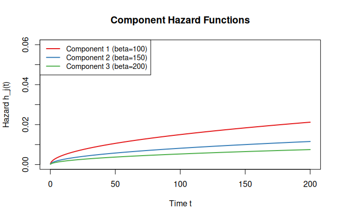

All three hazard curves are increasing ($k > 1$), but component 1 (smallest scale) has the steepest rate of increase and dominates at all times.

Cause probabilities

# Analytical cause weights: w_j = beta_j^{-k} / sum(beta_l^{-k})
w <- scales^(-k) / sum(scales^(-k))
names(w) <- paste0("Component ", 1:m)
cat("Cause weights (w_j):\n")
#> Cause weights (w_j):
print(round(w, 4))
#> Component 1 Component 2 Component 3 
#>      0.5269      0.2868      0.1863

The conditional_cause_probability() generic confirms these are time-invariant:

ccp_fn <- conditional_cause_probability(
  wei_series_homogeneous_md_c1_c2_c3(scales = scales)
)
probs <- ccp_fn(t_grid, theta)

plot(NULL, xlim = c(0, 200), ylim = c(0, 0.7),
     xlab = "Time t", ylab = "P(K = j | T = t)",
     main = "Conditional Cause Probability vs Time")
for (j in seq_len(m)) {
  lines(t_grid, probs[, j], col = cols[j], lwd = 2)
}
legend("right", paste0("Component ", 1:m),
       col = cols, lwd = 2, cex = 0.9)
abline(h = w, col = cols, lty = 3)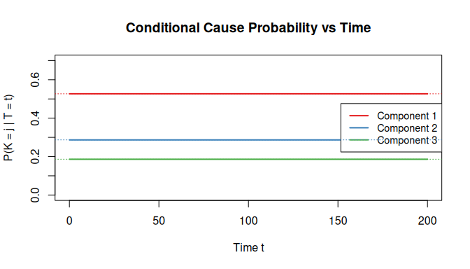

The conditional cause probabilities are flat lines, confirming that the homogeneous shape creates time-invariant cause attributions – a key structural simplification shared with the exponential model.

Data generation with periodic inspection

gen <- rdata(model)

set.seed(2024)
df <- gen(theta, n = 500, p = 0.3,
          observe = observe_periodic(delta = 20, tau = 250))

cat("Observation types:\n")
#> Observation types:
print(table(df$omega))
#> 
#> interval 
#>      500
cat("\nFirst 6 rows:\n")
#> 
#> First 6 rows:
print(head(df), row.names = FALSE)
#>    t    omega t_upper    x1    x2    x3
#>    0 interval      20 FALSE  TRUE  TRUE
#>  100 interval     120  TRUE FALSE FALSE
#>   40 interval      60  TRUE FALSE FALSE
#>   40 interval      60  TRUE FALSE  TRUE
#>   40 interval      60 FALSE  TRUE FALSE
#>   40 interval      60  TRUE FALSE  TRUE

Likelihood Contributions

The log-likelihood under conditions C1, C2, C3 decomposes into individual observation contributions. The homogeneous shape is critical: because the system lifetime is Weibull($k$, $\beta_{\text{sys}}$), left- and interval-censored terms have closed-form expressions involving only the system Weibull CDF and cause weights $w_c$.

Let $c_i$ denote the candidate set for observation $i$ and define $w_{c_i} = \sum_{j \in c_i} \beta_j^{-k} / \sum_l \beta_l^{-k}$.

Exact observation ($\omega_i = \text{exact}$)

The system failed at observed time $t_i$: $$\ell_i = \log\!\left(\sum_{j \in c_i} h_j(t_i)\right) - \sum_{j=1}^m \left(\frac{t_i}{\beta_j}\right)^k.$$

Right-censored ($\omega_i = \text{right}$)

The system survived past $t_i$ (no candidate set information): $$\ell_i = -\sum_{j=1}^m \left(\frac{t_i}{\beta_j}\right)^k = -\left(\frac{t_i}{\beta_{\text{sys}}}\right)^k.$$

Left-censored ($\omega_i = \text{left}$)

The system failed before inspection time $\tau_i$: $$\ell_i = \log w_{c_i} + \log\!\left( 1 - \exp\!\left(-\left(\frac{\tau_i}{\beta_{\text{sys}}}\right)^k\right) \right).$$ This is $\log w_{c_i} + \log F_{\text{sys}}(\tau_i)$, where $F_{\text{sys}}$ is the system Weibull CDF – a closed form that does not require numerical integration. The $w_{c_i}$ term arises because, under homogeneous shapes, the cause attribution and system lifetime factor cleanly.

Interval-censored ($\omega_i = \text{interval}$)

The system failed in $(a_i, b_i)$: $$\ell_i = \log w_{c_i} - \left(\frac{a_i}{\beta_{\text{sys}}}\right)^k + \log\!\left(1 - \exp\!\left( -\left(\left(\frac{b_i}{\beta_{\text{sys}}}\right)^k - \left(\frac{a_i}{\beta_{\text{sys}}}\right)^k\right) \right)\right).$$ This is $\log w_{c_i} + \log(R_{\text{sys}}(a_i) - R_{\text{sys}}(b_i))$, again in closed form.

Why homogeneous shapes enable closed forms

In the heterogeneous Weibull model (wei_series_md_c1_c2_c3), the system survival function $R_{\text{sys}}(t) = \prod_j \exp(-(t/\beta_j)^{k_j})$ does not reduce to a single Weibull, so the left- and interval-censored contributions require numerical integration via cubature. The homogeneous constraint $k_j = k$ for all $j$ collapses the product into a single Weibull CDF evaluation, and the cause weights $w_{c_i}$ separate from the time dependence. This makes the homogeneous model substantially faster and more numerically stable for censored data.

MLE Fitting

We fit the model to the periodically inspected data generated above using the fit() generic, which returns a solver based on optim:

solver <- fit(model)
theta0 <- c(1.2, 110, 140, 180)  # Initial guess near true values

estimate <- solver(df, par = theta0, method = "Nelder-Mead")
print(estimate)
#> Maximum Likelihood Estimate (Fisherian)
#> ----------------------------------------
#> Coefficients:
#> [1]   1.48 100.94 149.80 247.39
#> 
#> Log-likelihood: -1326 
#> Observations: 500

cat("True parameters: ", round(theta, 2), "\n")
#> True parameters:  1.5 100 150 200
cat("MLE estimates:   ", round(estimate$par, 2), "\n")
#> MLE estimates:    1.48 100.9 149.8 247.4
cat("Std errors:      ", round(sqrt(diag(estimate$vcov)), 2), "\n")
#> Std errors:       0.05 4.63 10.16 27.54
cat("Relative error:  ",
    round(100 * abs(estimate$par - theta) / theta, 1), "%\n")
#> Relative error:   1.4 0.9 0.1 23.7 %

Score and Hessian computation

The score function uses a hybrid approach: analytical gradients for exact and right-censored observations, and numDeriv::grad for left- and interval-censored observations. The Hessian is fully numerical, computed as the Jacobian of the score via numDeriv::jacobian.

ll_fn <- loglik(model)
scr_fn <- score(model)
hess_fn <- hess_loglik(model)

# Score at MLE should be near zero
scr_mle <- scr_fn(df, estimate$par)
cat("Score at MLE:", round(scr_mle, 4), "\n")
#> Score at MLE: -0.141 -0.0018 -1e-04 -2e-04

# Verify score against numerical gradient
scr_num <- numDeriv::grad(function(th) ll_fn(df, th), estimate$par)
cat("Max |analytical - numerical| score:",
    formatC(max(abs(scr_mle - scr_num)), format = "e", digits = 2), "\n")
#> Max |analytical - numerical| score: 0.00e+00

# Hessian eigenvalues (should be negative for concavity)
H <- hess_fn(df, estimate$par)
cat("Hessian eigenvalues:", round(eigen(H)$values, 2), "\n")
#> Hessian eigenvalues: -431 -0.05 -0.01 0

Monte Carlo Simulation Study

We compare estimation performance across three shape regimes: decreasing failure rate ($k = 0.7$), constant ($k = 1.0$), and increasing ($k = 1.5$). Each scenario uses $m = 3$ components, $n = 500$ observations, Bernoulli masking with $p = 0.3$, and periodic inspection with approximately 25% right-censoring.

set.seed(2024)

B <- 100          # Monte Carlo replications
n_mc <- 500       # Sample size per replication
p_mc <- 0.3       # Masking probability
alpha <- 0.05     # CI level

# Three shape regimes
scenarios <- list(
  DFR = c(k = 0.7, beta1 = 100, beta2 = 150, beta3 = 200),
  CFR = c(k = 1.0, beta1 = 100, beta2 = 150, beta3 = 200),
  IFR = c(k = 1.5, beta1 = 100, beta2 = 150, beta3 = 200)
)

results <- list()

model_mc <- wei_series_homogeneous_md_c1_c2_c3()
gen_mc <- rdata(model_mc)
solver_mc <- fit(model_mc)

for (sc_name in names(scenarios)) {
  th <- scenarios[[sc_name]]
  k_sc <- th[1]
  scales_sc <- th[-1]
  m_sc <- length(scales_sc)
  npars <- m_sc + 1

  # Choose tau to give ~25% right-censoring
  beta_sys_sc <- wei_series_system_scale(k_sc, scales_sc)
  tau_sc <- qweibull(0.75, shape = k_sc, scale = beta_sys_sc)
  delta_sc <- tau_sc / 10  # ~10 inspection intervals

  estimates <- matrix(NA, nrow = B, ncol = npars)
  se_est <- matrix(NA, nrow = B, ncol = npars)
  ci_lower <- matrix(NA, nrow = B, ncol = npars)
  ci_upper <- matrix(NA, nrow = B, ncol = npars)
  converged <- logical(B)
  cens_fracs <- numeric(B)

  for (b in seq_len(B)) {
    df_b <- gen_mc(th, n = n_mc, p = p_mc,
                   observe = observe_periodic(delta = delta_sc, tau = tau_sc))
    cens_fracs[b] <- mean(df_b$omega == "right")

    tryCatch({
      est_b <- solver_mc(df_b, par = c(1, rep(120, m_sc)),
                         method = "L-BFGS-B",
                         lower = rep(1e-6, npars))
      estimates[b, ] <- est_b$par
      se_est[b, ] <- sqrt(diag(est_b$vcov))
      z <- qnorm(1 - alpha / 2)
      ci_lower[b, ] <- est_b$par - z * se_est[b, ]
      ci_upper[b, ] <- est_b$par + z * se_est[b, ]
      converged[b] <- est_b$converged
    }, error = function(e) {
      converged[b] <<- FALSE
    })
  }

  results[[sc_name]] <- list(
    theta = th, estimates = estimates, se_est = se_est,
    ci_lower = ci_lower, ci_upper = ci_upper,
    converged = converged, cens_fracs = cens_fracs,
    tau = tau_sc, delta = delta_sc
  )
}

Bias and MSE by shape regime

summary_rows <- list()

for (sc_name in names(results)) {
  res <- results[[sc_name]]
  th <- res$theta
  valid <- res$converged & !is.na(res$estimates[, 1])
  est_v <- res$estimates[valid, , drop = FALSE]

  bias <- colMeans(est_v) - th
  variance <- apply(est_v, 2, var)
  mse <- bias^2 + variance
  pnames <- c("k", paste0("beta", seq_along(th[-1])))

  for (j in seq_along(th)) {
    summary_rows[[length(summary_rows) + 1]] <- data.frame(
      Regime = sc_name,
      Parameter = pnames[j],
      True = th[j],
      Mean_Est = mean(est_v[, j]),
      Bias = bias[j],
      RMSE = sqrt(mse[j]),
      Rel_Bias_Pct = 100 * bias[j] / th[j],
      stringsAsFactors = FALSE
    )
  }
}

mc_table <- do.call(rbind, summary_rows)

knitr::kable(mc_table, digits = 3, row.names = FALSE,
             caption = "Monte Carlo Results by Shape Regime (B=100, n=500)",
             col.names = c("Regime", "Parameter", "True", "Mean Est.",
                          "Bias", "RMSE", "Rel. Bias %"))

Monte Carlo Results by Shape Regime (B=100, n=500)

Regime	Parameter	True	Mean Est.	Bias	RMSE	Rel. Bias %
DFR	k	0.7	0.700	0.000	0.039	-0.046
DFR	beta1	100.0	102.108	2.108	16.190	2.108
DFR	beta2	150.0	156.849	6.849	29.900	4.566
DFR	beta3	200.0	208.930	8.930	46.026	4.465
CFR	k	1.0	0.997	-0.003	0.052	-0.329
CFR	beta1	100.0	102.388	2.388	11.367	2.388
CFR	beta2	150.0	151.217	1.217	21.640	0.811
CFR	beta3	200.0	205.608	5.608	30.815	2.804
IFR	k	1.5	1.503	0.003	0.064	0.231
IFR	beta1	100.0	100.785	0.785	6.674	0.785
IFR	beta2	150.0	150.996	0.996	13.150	0.664
IFR	beta3	200.0	201.455	1.455	24.228	0.728

Confidence interval coverage

coverage_rows <- list()

for (sc_name in names(results)) {
  res <- results[[sc_name]]
  th <- res$theta
  valid <- res$converged & !is.na(res$ci_lower[, 1])
  pnames <- c("k", paste0("beta", seq_along(th[-1])))

  for (j in seq_along(th)) {
    valid_j <- valid & !is.na(res$ci_lower[, j]) & !is.na(res$ci_upper[, j])
    covered <- (res$ci_lower[valid_j, j] <= th[j]) &
               (th[j] <= res$ci_upper[valid_j, j])
    width <- mean(res$ci_upper[valid_j, j] - res$ci_lower[valid_j, j])

    coverage_rows[[length(coverage_rows) + 1]] <- data.frame(
      Regime = sc_name,
      Parameter = pnames[j],
      Coverage = mean(covered),
      Mean_Width = width,
      stringsAsFactors = FALSE
    )
  }
}

cov_table <- do.call(rbind, coverage_rows)

knitr::kable(cov_table, digits = 3, row.names = FALSE,
             caption = "95% Wald CI Coverage by Shape Regime",
             col.names = c("Regime", "Parameter", "Coverage", "Mean Width"))

95% Wald CI Coverage by Shape Regime

Regime	Parameter	Coverage	Mean Width
DFR	k	0.949	0.150
DFR	beta1	0.949	60.773
DFR	beta2	0.960	115.664
DFR	beta3	0.970	176.434
CFR	k	0.950	0.193
CFR	beta1	0.940	39.604
CFR	beta2	0.900	76.988
CFR	beta3	0.980	127.453
IFR	k	0.980	0.275
IFR	beta1	0.950	22.968
IFR	beta2	0.950	52.617
IFR	beta3	0.950	92.139

Censoring rates

for (sc_name in names(results)) {
  res <- results[[sc_name]]
  conv_rate <- mean(res$converged)
  cens_rate <- mean(res$cens_fracs[res$converged])
  cat(sprintf("%s (k=%.1f): convergence=%.1f%%, mean censoring=%.1f%%\n",
              sc_name, res$theta[1], 100 * conv_rate, 100 * cens_rate))
}
#> DFR (k=0.7): convergence=99.0%, mean censoring=25.2%
#> CFR (k=1.0): convergence=100.0%, mean censoring=25.0%
#> IFR (k=1.5): convergence=100.0%, mean censoring=25.0%

Sampling distribution visualization

par(mfrow = c(3, 4), mar = c(4, 3, 2, 1), oma = c(0, 0, 2, 0))
pnames <- c("k", "beta1", "beta2", "beta3")

for (sc_name in names(results)) {
  res <- results[[sc_name]]
  th <- res$theta
  valid <- res$converged & !is.na(res$estimates[, 1])
  est_v <- res$estimates[valid, , drop = FALSE]

  for (j in seq_along(th)) {
    hist(est_v[, j], breaks = 20, probability = TRUE,
         main = paste0(sc_name, ": ", pnames[j]),
         xlab = pnames[j],
         col = "lightblue", border = "white", cex.main = 0.9)
    abline(v = th[j], col = "red", lwd = 2, lty = 2)
    abline(v = mean(est_v[, j]), col = "blue", lwd = 2)
  }
}

mtext("Sampling Distributions by Regime", outer = TRUE, cex = 1.2)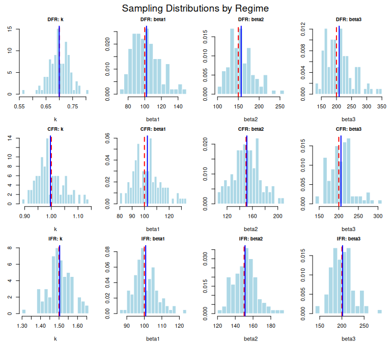

Interpretation

The Monte Carlo study reveals several patterns:

• Shape estimation accuracy varies by regime. In absolute terms, the DFR regime ($k = 0.7$) has the smallest shape RMSE, while IFR ($k = 1.5$) has the best relative precision (RMSE/$k$). IFR has the widest absolute confidence intervals simply because the parameter value is largest; the relative CI width (width/$k$) is actually smallest for IFR. The steeper curvature of the IFR hazard function provides stronger signal about the shape parameter relative to its magnitude.

• Scale estimation is robust across regimes. Relative bias in the scale parameters is below 5% in all three regimes. Coverage is near the nominal 95% for most parameters, though a few (e.g., CFR $\beta_2$) show undercoverage around 90%, which is borderline significant at $B = 100$ replications. In the DFR regime, scale parameters exhibit positive bias that increases with the true scale value.

• Periodic inspection adds interval-censoring. Unlike the exponential vignette which used only exact + right observations, this study uses periodic inspection. The closed-form interval-censored contributions (unique to the homogeneous model) keep computation fast despite the additional complexity.

Weibull($k=1$) = Exponential Identity

When $k = 1$, the homogeneous Weibull model reduces to the exponential model. We verify this numerically by comparing log-likelihoods on the same data.

# Parameters: k=1 with scales equivalent to rates (1/beta_j)
exp_rates <- c(0.01, 0.008, 0.005)
wei_scales <- 1 / exp_rates  # beta = 1/lambda
wei_theta <- c(1, wei_scales)

# Generate data under exponential model
exp_model <- exp_series_md_c1_c2_c3()
exp_gen <- rdata(exp_model)

set.seed(42)
df_test <- exp_gen(exp_rates, n = 200, tau = 300, p = 0.3)

# Evaluate both log-likelihoods
ll_exp <- loglik(exp_model)
ll_wei <- loglik(model)

val_exp <- ll_exp(df_test, exp_rates)
val_wei <- ll_wei(df_test, wei_theta)

cat("Exponential loglik:", round(val_exp, 6), "\n")
#> Exponential loglik: -1104
cat("Weibull(k=1) loglik:", round(val_wei, 6), "\n")
#> Weibull(k=1) loglik: -1104
cat("Absolute difference:", formatC(abs(val_exp - val_wei),
                                     format = "e", digits = 2), "\n")
#> Absolute difference: 2.27e-13

The two log-likelihoods agree to machine precision, confirming that the homogeneous Weibull model is a proper generalization of the exponential series model. This also serves as a consistency check on the implementation.

# Score comparison
s_exp <- score(exp_model)(df_test, exp_rates)
s_wei <- score(model)(df_test, wei_theta)

# The exponential score is d/d(lambda_j), the Weibull score includes d/dk
# and d/d(beta_j). Since lambda_j = 1/beta_j, by the chain rule:
#   d(ell)/d(lambda_j) = d(ell)/d(beta_j) * d(beta_j)/d(lambda_j)
#                      = d(ell)/d(beta_j) * (-beta_j^2)
# So: d(ell)/d(lambda_j) = -beta_j^2 * d(ell)/d(beta_j)
s_wei_transformed <- -wei_scales^2 * s_wei[-1]

cat("Exponential score:        ", round(s_exp, 4), "\n")
#> Exponential score:         -1490 -395 -439.4
cat("Weibull(k=1) scale score: ", round(s_wei_transformed, 4), "\n")
#> Weibull(k=1) scale score:  -1490 -395 -439.4
cat("Max |difference|:",
    formatC(max(abs(s_exp - s_wei_transformed)), format = "e", digits = 2), "\n")
#> Max |difference|: 1.48e-12

The transformed Weibull scale scores match the exponential rate scores to machine precision, confirming that the two parameterizations yield identical inference at $k = 1$. The shape score $\partial\ell/\partial k$ is nonzero at the true parameter (the score is zero only at the MLE, not at the DGP truth for any finite sample).