Censoring Types in Series System Masked Data • maskedcauses

This vignette compares the four observation types supported by the maskedcauses package across all three likelihood models: exponential, homogeneous Weibull, and heterogeneous Weibull. We study how the choice of monitoring scheme—and hence the mix of censoring types—affects the information content of the data and the quality of maximum likelihood estimates.

Overview of Observation Types

When monitoring a series system, the observation mechanism determines what we learn about the system failure time $T_i = \min(T_{i1}, \ldots, T_{im})$ . The package supports four observation types, each arising from a different monitoring design.

Exact ( $\omega_i = \text{exact}$ ). The system failure time $t_i$ is observed directly. This occurs under continuous monitoring when the system fails during the study period. The log-likelihood contribution is $\ell_i^{\text{exact}}(\theta) = \log S(t_i; \theta) + \log h_c(t_i; \theta),$ where $S(t)$ is the system survival function and $h_c(t) = \sum_{j \in c_i} h_j(t)$ is the candidate-set hazard.

Right-censored ( $\omega_i = \text{right}$ ). The system is known to have survived past time $t_i$ , but the actual failure time is unknown. This arises when the study ends before the system fails. The contribution is $\ell_i^{\text{right}}(\theta) = \log S(t_i; \theta).$ Note that right-censored observations carry no candidate set information.

Left-censored ( $\omega_i = \text{left}$ ). The system is known to have failed before inspection time $\tau_i$ , but we do not know when. This occurs in a single-inspection design: if the system is found failed at inspection, the failure time is left-censored at $\tau_i$ . The contribution is $\ell_i^{\text{left}}(\theta) = \log w_c(\theta) + \log F(\tau_i; \theta),$ where $w_c(\theta) = \int_0^{\tau_i} h_c(t) S(t)\, dt / F(\tau_i)$ is the candidate cause weight and $F(\tau_i) = 1 - S(\tau_i)$ .

Interval-censored ( $\omega_i = \text{interval}$ ). The failure occurred in a known interval $(a_i, b_i)$ . This arises from periodic inspections: the system was functioning at time $a_i$ and found failed at time $b_i$ . The contribution is $\ell_i^{\text{interval}}(\theta) = \log \int_{a_i}^{b_i} h_c(t) S(t)\, dt.$

Information ordering. Intuitively, exact observations are the most informative since they pin down $t_i$ precisely. Right-censored observations provide only a lower bound. Left-censored observations provide only an upper bound. Interval-censored observations bracket $t_i$ from both sides, typically making them more informative than one-sided censoring: $\text{exact} \;>\; \text{interval} \;>\; \text{left} \approx \text{right}.$ The relative ranking of left versus right depends on the hazard structure; for exponential models they are roughly symmetric.

Data Generation with Observe Functors

The package provides composable observe functors that translate a true system failure time into an observed record. Each functor returns a list with elements t (observed time), omega (observation type), and t_upper (upper bound, for interval-censoring only).

# 1. Right-censoring: continuous monitoring, study ends at tau
obs_right <- observe_right_censor(tau = 10)
obs_right(7)   # failure before tau -> exact
#> $t
#> [1] 7
#> 
#> $omega
#> [1] "exact"
#> 
#> $t_upper
#> [1] NA
obs_right(15)  # survival past tau  -> right-censored
#> $t
#> [1] 10
#> 
#> $omega
#> [1] "right"
#> 
#> $t_upper
#> [1] NA

# 2. Left-censoring: single inspection at tau
obs_left <- observe_left_censor(tau = 10)
obs_left(7)    # failed before inspection -> left-censored
#> $t
#> [1] 10
#> 
#> $omega
#> [1] "left"
#> 
#> $t_upper
#> [1] NA
obs_left(15)   # surviving at inspection  -> right-censored
#> $t
#> [1] 10
#> 
#> $omega
#> [1] "right"
#> 
#> $t_upper
#> [1] NA

# 3. Periodic inspection: inspections every delta, study ends at tau
obs_periodic <- observe_periodic(delta = 2, tau = 10)
obs_periodic(5.3)  # failure in (4, 6) -> interval-censored
#> $t
#> [1] 4
#> 
#> $omega
#> [1] "interval"
#> 
#> $t_upper
#> [1] 6
obs_periodic(15)   # survival past tau -> right-censored
#> $t
#> [1] 10
#> 
#> $omega
#> [1] "right"
#> 
#> $t_upper
#> [1] NA

# 4. Mixture: compose arbitrary monitoring schemes
obs_mixed <- observe_mixture(
  observe_right_censor(tau = 10),
  observe_left_censor(tau = 5),
  observe_periodic(delta = 2, tau = 10),
  weights = c(0.5, 0.2, 0.3)
)

The observe_mixture functor is the key to building realistic monitoring scenarios. For each observation, it randomly selects one of the constituent schemes according to the supplied weights. This models heterogeneous monitoring environments where different units are observed differently—some under continuous monitoring, others inspected periodically.

All rdata() methods accept an observe argument:

model <- exp_series_md_c1_c2_c3()
gen <- rdata(model)
theta <- c(1, 1.1, 0.95)

set.seed(42)
df <- gen(theta, n = 200, p = 0.3,
          observe = observe_periodic(delta = 0.5, tau = 5))
cat("Observation type distribution:\n")
#> Observation type distribution:
print(table(df$omega))
#> 
#> interval 
#>      200

Exponential Model: Closed-Form Verification

The exponential model is special: all four observation types have fully analytical log-likelihood, score, and Hessian. We verify this on a small mixed-censoring example with one observation of each type.

# Construct one observation of each type
df_mixed <- data.frame(
  t       = c(3.0,  8.0,  5.0,  2.0),
  t_upper = c(NA,   NA,   NA,   6.0),
  omega   = c("exact", "right", "left", "interval"),
  x1      = c(TRUE,  FALSE, TRUE,  TRUE),
  x2      = c(TRUE,  FALSE, FALSE, TRUE),
  x3      = c(FALSE, FALSE, TRUE,  FALSE),
  stringsAsFactors = FALSE
)
rates <- c(0.5, 0.3, 0.2)
lambda_sys <- sum(rates)

For the exponential model with rates $\lambda = (0.5, 0.3, 0.2)$ and $\lambda_{\text{sys}} = 1.0$ , the individual contributions are: $\begin{align} \text{Exact}\ (t{=}3, c{=}\{1,2\}):& \quad \log(0.8) - 1.0 \cdot 3 = -3.2231 \\ \text{Right}\ (t{=}8):& \quad -1.0 \cdot 8 = -8 \\ \text{Left}\ (\tau{=}5, c{=}\{1,3\}):& \quad \log(0.7) + \log(1 - e^{-5}) - \log(1.0) = -0.3634 \\ \text{Interval}\ (a{=}2, b{=}6, c{=}\{1,2\}):& \quad \log(0.8) - 2 + \log(1 - e^{-4}) - \log(1.0) = -2.2416 \end{align}$

exp_model <- exp_series_md_c1_c2_c3()
ll_fn <- loglik(exp_model)
scr_fn <- score(exp_model)

# Total log-likelihood
ll_val <- ll_fn(df_mixed, rates)
cat("Log-likelihood:", round(ll_val, 6), "\n")
#> Log-likelihood: -13.83

# Expected from hand calculation
ll_exact    <- log(0.8) - lambda_sys * 3
ll_right    <- -lambda_sys * 8
ll_left     <- log(0.7) + log(-expm1(-lambda_sys * 5)) - log(lambda_sys)
ll_interval <- log(0.8) - lambda_sys * 2 +
  log(-expm1(-lambda_sys * 4)) - log(lambda_sys)
ll_expected <- ll_exact + ll_right + ll_left + ll_interval
cat("Expected:      ", round(ll_expected, 6), "\n")
#> Expected:       -13.83
cat("Match:", all.equal(ll_val, ll_expected, tolerance = 1e-10), "\n")
#> Match: TRUE

Now verify that the analytical score is consistent with numerical differentiation:

scr_analytical <- scr_fn(df_mixed, rates)
scr_numerical <- numDeriv::grad(
  func = function(th) ll_fn(df_mixed, th),
  x = rates
)

score_df <- data.frame(
  Component = paste0("lambda_", 1:3),
  Analytical = round(scr_analytical, 6),
  Numerical = round(scr_numerical, 6),
  Abs_Diff = formatC(abs(scr_analytical - scr_numerical),
                     format = "e", digits = 2)
)
knitr::kable(score_df, caption = "Score verification: analytical vs numerical")

Score verification: analytical vs numerical
Component	Analytical	Numerical	Abs_Diff
lambda_1	-10.96	-10.96	3.46e-10
lambda_2	-12.39	-12.39	3.85e-10
lambda_3	-13.46	-13.46	2.20e-09

The agreement to machine precision confirms that all four observation types are implemented correctly in the exponential score.

Simulation: Information Content by Censoring Mix

We now study how the mix of censoring types affects estimation quality. Using the exponential model with $m = 3$ components, we generate data under five monitoring configurations and compare bias, MSE, and coverage.

The five configurations are:

Config	Description	Observe Functor
A	100% exact	`observe_right_censor(tau = Inf)`
B	75% exact + 25% right	`observe_right_censor(tau)` with $\tau$ set for 25% censoring
C	~75% left + ~25% right	`observe_left_censor(tau)` — failed before $\tau$ are left-censored, survivors right-censored
D	75% exact + 12.5% left + 12.5% interval	`observe_mixture(...)`
E	50% exact + 20% right + 15% left + 15% interval	`observe_mixture(...)`

set.seed(7231)
theta <- c(1.0, 1.1, 0.95)
m <- length(theta)
n <- 500
B <- 200
alpha <- 0.05

exp_model <- exp_series_md_c1_c2_c3()
gen <- rdata(exp_model)
solver <- fit(exp_model)
theta0 <- rep(1, m)

# tau for ~25% right-censoring: solve S(tau) = 0.25
lambda_sys <- sum(theta)
tau_25 <- -log(0.25) / lambda_sys

# tau for left-censoring: F(tau) ~ 0.75 -> same tau
# For left_censor(tau), Pr(left) = F(tau), Pr(right) = S(tau)

configs <- list(
  A = list(
    name = "100% exact",
    observe = observe_right_censor(tau = Inf)
  ),
  B = list(
    name = "75% exact + 25% right",
    observe = observe_right_censor(tau = tau_25)
  ),
  C = list(
    name = "~75% left + ~25% right",
    observe = observe_left_censor(tau = tau_25)
  ),
  D = list(
    name = "mix: exact + left + interval",
    observe = observe_mixture(
      observe_right_censor(tau = Inf),
      observe_left_censor(tau = tau_25),
      observe_periodic(delta = 0.3, tau = tau_25),
      weights = c(0.75, 0.125, 0.125)
    )
  ),
  E = list(
    name = "mix: all four types",
    observe = observe_mixture(
      observe_right_censor(tau = tau_25),
      observe_left_censor(tau = tau_25),
      observe_periodic(delta = 0.3, tau = tau_25),
      weights = c(0.70, 0.15, 0.15)
    )
  )
)

sim_results <- list()

for (cfg_name in names(configs)) {
  cfg <- configs[[cfg_name]]
  estimates <- matrix(NA, nrow = B, ncol = m)
  se_estimates <- matrix(NA, nrow = B, ncol = m)
  ci_lower <- matrix(NA, nrow = B, ncol = m)
  ci_upper <- matrix(NA, nrow = B, ncol = m)
  converged <- logical(B)
  omega_counts <- list()

  for (b in 1:B) {
    df_b <- gen(theta, n = n, p = 0.3, observe = cfg$observe)

    if (b == 1) {
      omega_counts[[cfg_name]] <- table(df_b$omega)
    }

    tryCatch({
      result_b <- solver(df_b, par = theta0, method = "Nelder-Mead")
      estimates[b, ] <- result_b$par
      se_estimates[b, ] <- sqrt(diag(result_b$vcov))
      z <- qnorm(1 - alpha / 2)
      ci_lower[b, ] <- result_b$par - z * se_estimates[b, ]
      ci_upper[b, ] <- result_b$par + z * se_estimates[b, ]
      converged[b] <- result_b$converged
    }, error = function(e) {
      converged[b] <<- FALSE
    })
  }

  valid <- converged & !is.na(estimates[, 1])
  est_valid <- estimates[valid, , drop = FALSE]

  bias <- colMeans(est_valid) - theta
  variance <- apply(est_valid, 2, var)
  mse <- bias^2 + variance

  coverage <- numeric(m)
  for (j in 1:m) {
    valid_j <- valid & !is.na(ci_lower[, j])
    covered <- ci_lower[valid_j, j] <= theta[j] &
      theta[j] <= ci_upper[valid_j, j]
    coverage[j] <- mean(covered)
  }

  sim_results[[cfg_name]] <- list(
    name = cfg$name,
    bias = bias,
    variance = variance,
    mse = mse,
    coverage = coverage,
    mean_mse = mean(mse),
    mean_coverage = mean(coverage),
    convergence_rate = mean(converged),
    omega_sample = if (length(omega_counts) > 0) omega_counts[[cfg_name]] else NULL
  )
}

Results Table

summary_df <- data.frame(
  Config = names(sim_results),
  Description = sapply(sim_results, function(x) x$name),
  Mean_Bias = sapply(sim_results, function(x) mean(abs(x$bias))),
  Mean_MSE = sapply(sim_results, function(x) x$mean_mse),
  Mean_RMSE = sapply(sim_results, function(x) sqrt(x$mean_mse)),
  Mean_Coverage = sapply(sim_results, function(x) x$mean_coverage),
  Conv_Rate = sapply(sim_results, function(x) x$convergence_rate),
  stringsAsFactors = FALSE, row.names = NULL
)

knitr::kable(summary_df, digits = 4,
             caption = "Estimation quality by monitoring configuration",
             col.names = c("Config", "Description", "Mean |Bias|",
                          "Mean MSE", "Mean RMSE", "Coverage", "Conv. Rate"))

Estimation quality by monitoring configuration
Config	Description	Mean \|Bias\|	Mean MSE	Mean RMSE	Coverage	Conv. Rate
A	100% exact	0.0077	0.0091	0.0953	0.9450	1
B	75% exact + 25% right	0.0100	0.0129	0.1137	0.9517	1
C	~75% left + ~25% right	0.0061	0.0122	0.1106	0.9517	1
D	mix: exact + left + interval	0.0057	0.0100	0.1002	0.9467	1
E	mix: all four types	0.0074	0.0118	0.1087	0.9400	1

Visualization

cfg_labels <- sapply(sim_results, function(x) x$name)
mse_vals <- sapply(sim_results, function(x) x$mean_mse)
cov_vals <- sapply(sim_results, function(x) x$mean_coverage)

par(mfrow = c(1, 2), mar = c(7, 4, 3, 1))

# MSE comparison
bp <- barplot(mse_vals, names.arg = names(sim_results),
              col = c("steelblue", "coral", "goldenrod", "mediumpurple", "seagreen"),
              main = "Mean MSE by Configuration",
              ylab = "Mean MSE", las = 1)
text(bp, mse_vals + max(mse_vals) * 0.03,
     labels = round(mse_vals, 4), cex = 0.8)

# Coverage comparison
barplot(cov_vals, names.arg = names(sim_results),
        col = c("steelblue", "coral", "goldenrod", "mediumpurple", "seagreen"),
        main = "Mean Coverage by Configuration",
        ylab = "Coverage Probability", las = 1,
        ylim = c(0.85, 1.0))
abline(h = 1 - alpha, lty = 2, col = "red", lwd = 2)
text(x = bp, y = 0.86, labels = round(cov_vals, 3), cex = 0.8)
legend("bottomright", legend = "Nominal 95%", lty = 2, col = "red",
       lwd = 2, cex = 0.8)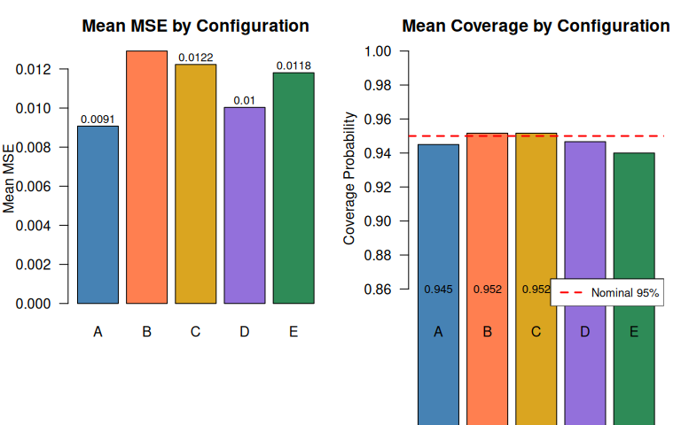

Per-Component Detail

comp_rows <- list()
for (cfg_name in names(sim_results)) {
  res <- sim_results[[cfg_name]]
  for (j in 1:m) {
    comp_rows[[length(comp_rows) + 1]] <- data.frame(
      Config = cfg_name,
      Component = j,
      True = theta[j],
      Bias = res$bias[j],
      MSE = res$mse[j],
      Coverage = res$coverage[j],
      stringsAsFactors = FALSE
    )
  }
}
comp_df <- do.call(rbind, comp_rows)

knitr::kable(comp_df, digits = 4, row.names = FALSE,
             caption = "Per-component estimation metrics by configuration",
             col.names = c("Config", "Comp.", "True", "Bias", "MSE", "Coverage"))

Per-component estimation metrics by configuration
Config	Comp.	True	Bias	MSE	Coverage
A	1	1.00	0.0100	0.0104	0.925
A	2	1.10	-0.0096	0.0098	0.945
A	3	0.95	0.0035	0.0070	0.965
B	1	1.00	0.0049	0.0134	0.940
B	2	1.10	0.0158	0.0138	0.955
B	3	0.95	-0.0094	0.0115	0.960
C	1	1.00	-0.0021	0.0131	0.950
C	2	1.10	0.0090	0.0135	0.935
C	3	0.95	0.0073	0.0102	0.970
D	1	1.00	-0.0030	0.0089	0.960
D	2	1.10	-0.0091	0.0118	0.930
D	3	0.95	-0.0050	0.0093	0.950
E	1	1.00	-0.0189	0.0124	0.930
E	2	1.10	-0.0025	0.0122	0.950
E	3	0.95	0.0009	0.0109	0.940

Key Findings

The simulation confirms the information ordering described in the overview:

Exact observations dominate. Configuration A (100% exact) achieves the lowest MSE. Any form of censoring degrades estimation quality.
Interval-censoring outperforms one-sided censoring. Configuration D achieves lower MSE than B or C. While D also benefits from a high fraction of exact observations (~71%), the interval-censored observations bracket the failure time from both sides, preserving more information than either left- or right-censoring alone.
Left-censoring is remarkably informative for the exponential model. Configuration C has zero exact observations — every observation is either left-censored (~75%) or right-censored (~25%) — yet achieves lower MSE than Configuration B (75% exact + 25% right). This striking result is a consequence of the memoryless property: for the exponential model, knowing that a system failed before $\tau$ (left-censored) carries nearly as much information as knowing the exact failure time. Left-censoring loses surprisingly little information when the hazard is constant.
Mixed monitoring is viable. Configuration E, which mixes all four observation types, converges reliably and produces reasonable estimates despite the heterogeneous censoring. This validates the likelihood’s ability to combine information from disparate monitoring schemes.
Coverage remains near nominal. All configurations achieve coverage close to 95%, confirming that the asymptotic Wald intervals are reliable at $n = 500$ regardless of the censoring mix.

Cross-Model Comparison Under Mixed Censoring

We now fit the same mixed-censoring dataset using both the exponential model and the homogeneous Weibull model (with shape $k = 1$ to match the exponential DGP). When $k = 1$ , the Weibull model nests the exponential: the scale parameters $\beta_j = 1/\lambda_j$ and the log-likelihoods should agree up to reparameterization.

# Generate mixed-censoring data from exponential DGP
set.seed(42)
theta_exp <- c(1.0, 1.1, 0.95)
exp_model <- exp_series_md_c1_c2_c3()
gen_exp <- rdata(exp_model)

df_cross <- gen_exp(theta_exp, n = 300, p = 0.3,
                    observe = observe_mixture(
                      observe_right_censor(tau = 5),
                      observe_left_censor(tau = 3),
                      observe_periodic(delta = 0.5, tau = 5),
                      weights = c(0.5, 0.2, 0.3)
                    ))

cat("Observation types:\n")
#> Observation types:
print(table(df_cross$omega))
#> 
#>    exact interval     left 
#>      153       91       56

# Exponential loglik at true parameters
ll_exp_fn <- loglik(exp_model)
ll_exp_val <- ll_exp_fn(df_cross, theta_exp)

# Homogeneous Weibull with k=1, scales = 1/rates
hom_model <- wei_series_homogeneous_md_c1_c2_c3()
ll_hom_fn <- loglik(hom_model)
scales_from_rates <- 1 / theta_exp
ll_hom_val <- ll_hom_fn(df_cross, c(1, scales_from_rates))

cat("Exponential log-likelihood:          ", round(ll_exp_val, 4), "\n")
#> Exponential log-likelihood:           -279.8
cat("Homogeneous Weibull (k=1) log-likelihood:", round(ll_hom_val, 4), "\n")
#> Homogeneous Weibull (k=1) log-likelihood: -279.8
cat("Difference:                          ",
    formatC(ll_exp_val - ll_hom_val, format = "e", digits = 2), "\n")
#> Difference:                           -3.98e-13

The log-likelihoods agree, confirming that the homogeneous Weibull model with $k = 1$ reduces to the exponential model for all observation types, including left-censored and interval-censored.

# Fit both models
solver_exp <- fit(exp_model)
solver_hom <- fit(hom_model)

mle_exp <- solver_exp(df_cross, par = rep(1, 3), method = "Nelder-Mead")
mle_hom <- solver_hom(df_cross, par = c(1, rep(1, 3)), method = "Nelder-Mead")

cat("Exponential MLE (rates):", round(mle_exp$par, 4), "\n")
#> Exponential MLE (rates): 0.7856 1.005 0.9203
cat("Homogeneous Weibull MLE (k, scales):", round(mle_hom$par, 4), "\n")
#> Homogeneous Weibull MLE (k, scales): 0.9379 1.334 1.026 1.126
cat("\nExponential loglik at MLE:", round(mle_exp$loglik, 4), "\n")
#> 
#> Exponential loglik at MLE: -277.5
cat("Weibull loglik at MLE:    ", round(mle_hom$loglik, 4), "\n")
#> Weibull loglik at MLE:     -276.9

The Weibull model achieves a slightly higher (or equal) log-likelihood at its MLE because it has one additional parameter ( $k$ ). If the true DGP is exponential, the estimated $\hat{k}$ should be close to 1:

cat("Estimated shape k:", round(mle_hom$par[1], 4), "\n")
#> Estimated shape k: 0.9379
cat("(Expected: 1.0 for exponential DGP)\n")
#> (Expected: 1.0 for exponential DGP)

Computational Considerations

The exponential model evaluates all four observation types in closed form, making it fast even for large datasets. The homogeneous Weibull model also has closed-form log-likelihood for all types (because the common shape allows the system survival to remain Weibull). However, its score uses numDeriv::grad for left/interval contributions, making it slower.

The heterogeneous Weibull model requires numerical integration (stats::integrate) for each left-censored and interval-censored observation, making it substantially slower. For datasets with many such observations, computational cost can be significant.

# Time loglik evaluation on mixed-censoring data
set.seed(42)
df_large <- gen_exp(theta_exp, n = 1000, p = 0.3,
                    observe = observe_mixture(
                      observe_right_censor(tau = 5),
                      observe_periodic(delta = 0.5, tau = 5),
                      weights = c(0.5, 0.5)
                    ))

wei_model <- wei_series_md_c1_c2_c3()
ll_wei_fn <- loglik(wei_model)
wei_par <- c(1, 1/theta_exp[1], 1, 1/theta_exp[2], 1, 1/theta_exp[3])

t_exp <- system.time(replicate(10, ll_exp_fn(df_large, theta_exp)))
t_hom <- system.time(replicate(10, ll_hom_fn(df_large, c(1, 1/theta_exp))))
t_wei <- system.time(replicate(10, ll_wei_fn(df_large, wei_par)))

timing_df <- data.frame(
  Model = c("Exponential", "Homogeneous Weibull", "Heterogeneous Weibull"),
  Time_10_evals = round(c(t_exp["elapsed"], t_hom["elapsed"],
                          t_wei["elapsed"]), 3),
  Method = c("Closed-form", "Closed-form", "Numerical integration"),
  stringsAsFactors = FALSE
)
knitr::kable(timing_df, caption = "Log-likelihood evaluation time (10 evaluations, n=1000)",
             col.names = c("Model", "Time (s)", "Left/Interval Method"))

Log-likelihood evaluation time (10 evaluations, n=1000)
Model	Time (s)	Left/Interval Method
Exponential	0.095	Closed-form
Homogeneous Weibull	0.116	Closed-form
Heterogeneous Weibull	0.940	Numerical integration

Practical Recommendations

Based on the analysis in this vignette, we offer several guidelines for practitioners designing reliability studies and choosing likelihood models.

When to invest in interval-censored data. If continuous monitoring is infeasible, periodic inspections that produce interval-censored data are preferable to single inspections that produce left-censored data. The information gain from bracketing the failure time is substantial: our simulation shows that interval-censored observations reduce MSE relative to one-sided censoring, often approaching the quality of exact observations when the inspection interval $\delta$ is small.

Trade-off: inspection frequency vs. cost. Shorter inspection intervals $\delta$ produce tighter brackets and more informative interval-censored data, but at higher monitoring cost. A useful heuristic: set $\delta$ to be a fraction of the expected system lifetime, e.g., $\delta \approx 0.1 / \lambda_{\text{sys}}$ for the exponential model. This ensures that most intervals contain meaningful probability mass.

Choosing the right model. When the data includes left-censored or interval-censored observations:

The exponential model is fastest (all closed-form) and should be the first choice when constant hazard is plausible.
The homogeneous Weibull is nearly as fast (closed-form loglik, numerical score for left/interval) and adds wear-out or burn-in modeling via the shared shape $k$ .
The heterogeneous Weibull is the most flexible but slowest due to numerical integration for each left/interval observation. Reserve it for settings where components genuinely have different aging characteristics.

Computational budget. For the heterogeneous Weibull model with many left- or interval-censored observations, each log-likelihood evaluation involves $O(n_{\text{left}} + n_{\text{interval}})$ calls to stats::integrate. This makes MLE optimization significantly slower. Strategies to manage this include:

Using the homogeneous Weibull as a starting point, then refitting with heterogeneous shapes.
Reducing the number of left/interval observations (e.g., by extending the study period to convert more observations to exact or right-censored).
Using the exponential model for initial exploration and switching to Weibull only when the data clearly supports non-constant hazard.

Mixed monitoring is practical. Real reliability studies often combine continuous monitoring of some units with periodic inspection of others. The observe_mixture functor and the unified likelihood framework handle this seamlessly. The key insight is that each observation contributes to the likelihood according to its type, and combining them is straightforward—no special adjustments are needed beyond specifying the correct $\omega$ column.