Model Selection for Reliability Estimation in Series Systems
Abstract
When can reliability engineers safely use a simpler model for series system analysis? This paper provides a definitive answer: for well-designed systems with similar component failure characteristics, a reduced homogeneous-shape Weibull model is statistically indistinguishable from the full heterogeneous model even with 30,000 observations. This striking finding means practitioners can confidently use the simpler model—which halves the parameter count from to and renders the system itself Weibull-distributed—without sacrificing accuracy. However, our likelihood ratio tests reveal that deviations in even a single component’s shape parameter quickly provide evidence against the reduced model, offering clear guidance on when complexity is warranted. Using simulation studies with right-censored and masked failure data, we characterize the boundary between these regimes across sample sizes from 50 to 30,000 and shape parameter deviations from 0.25 to 3.0. The results provide actionable model selection guidance for reliability assessment under realistic data limitations.
1 Introduction
Estimating reliability of individual components in multi-component systems is challenging when only system-level failure data is observable. This problem arises frequently in industrial settings where diagnosing the exact cause of system failure is expensive or infeasible, resulting in masked failure data where only a candidate set of possible failure causes is known [4].
1.1 Related Work
The statistical treatment of masked system failure data has a substantial history. Usher and Hodgson [12] introduced maximum likelihood methods for component reliability estimation from masked system life-test data, establishing the foundational framework for this field. Lin, Usher, and Guess [13] extended this work to derive exact maximum likelihood estimators, while Lin, Usher, and Guess [6] developed Bayesian approaches for component reliability estimation from masked data.
For Weibull-distributed components specifically, Usher [14] addressed component reliability prediction in the presence of masked data. Guess and Usher [3] proposed an iterative approach for estimating component reliability that handles the computational challenges of masked data likelihood functions.
Sarhan [7] examined reliability estimation from masked system life data under various distributional assumptions, later extending this work to linear failure rate models [8]. Tan [9, 10] contributed methods for exponential component reliability estimation from masked binomial system testing data and uncertain life data in series and parallel systems. More recently, Guo, Niu, and Szidarovszky [5] studied estimating component reliabilities from incomplete system failure data, providing the baseline system configuration used in our simulation studies.
Building on this literature, Towell [11] developed a comprehensive likelihood model that incorporates both right-censoring and candidate sets for series systems with Weibull components, along with extensive simulation studies validating the maximum likelihood approach. The present paper extends that work by investigating model selection—specifically, when a reduced model assuming homogeneous component shapes is appropriate.
1.2 Contributions and Organization
This paper addresses a fundamental question in reliability engineering: when is a simpler model adequate? Among the possible simplifications of a full heterogeneous Weibull series model, the homogeneous-shape reduction is uniquely compelling: it is the only single-parameter constraint that renders the system lifetime itself Weibull, and it naturally captures the physical structure of well-designed systems where components share similar aging behavior but differ in absolute durability. The key contributions are:
-
1.
A striking robustness result: For well-designed series systems, the reduced homogeneous-shape model cannot be rejected even with sample sizes approaching 30,000—far larger than typically available in practice. This provides strong justification for using the simpler model.
-
2.
Sharp sensitivity boundaries: We quantify exactly how much component heterogeneity is needed before the likelihood ratio test rejects the reduced model, across a range of sample sizes and shape parameter values.
-
3.
Practical model selection guidance: Our results translate directly into actionable recommendations for practitioners facing the bias-variance tradeoff in reliability assessment.
The remainder of this paper is organized as follows. Section 2 presents mathematical preliminaries including formal notation, series system definitions, Weibull distribution properties, and foundational theorems. Section 3 summarizes the likelihood model for masked and censored data. Section 4 presents simulation studies assessing estimator sensitivity to system design variations. Section 5 introduces the reduced homogeneous shape model and evaluates its appropriateness using likelihood ratio tests. Section 6 concludes with practical guidance on model selection.
2 Mathematical Preliminaries
2.1 Notation and System Structure
Consider a series system composed of components, where the system fails when any single component fails. We observe independent and identically distributed system lifetimes. For the -th system (), let denote the lifetime of component (). The system lifetime is given by
| (1) |
We denote the complete parameter vector by , where is the shape parameter and is the scale parameter for component . Bold symbols represent vectors throughout this paper.
2.2 Weibull Distribution
Each component lifetime follows a two-parameter Weibull distribution with probability density function
| (2) |
reliability function
| (3) |
and hazard function
| (4) |
The mean time to failure (MTTF) for a Weibull-distributed component is
| (5) |
where is the gamma function. The shape parameter characterizes the failure mode:
-
•
If , the hazard function decreases with time, indicating infant mortality or early-life failures.
-
•
If , the hazard function is constant, corresponding to an exponential distribution with memoryless failures.
-
•
If , the hazard function increases with time, indicating wear-out or aging failures.
2.3 Data Structure
The observed data for each system consists of:
-
•
Observed system lifetime : The time at which system fails or is censored.
-
•
Censoring indicator : Equals 1 if system failed and 0 if right-censored.
-
•
Candidate set : For failed systems (), the set of components that could have caused the failure. For censored systems, is undefined.
This data structure is termed masked data because the true component cause of failure is not directly observed but is known to belong to the candidate set . The masking mechanism assumes that:
-
1.
The candidate set always contains the true failed component.
-
2.
Given the system failure time and the true failed component, the masking mechanism is non-informative, meaning the process generating candidate sets is independent of the parameter vector . For a detailed treatment of these conditions, see [11].
2.4 Well-Designed Systems
A well-designed series system is characterized by components having similar but not necessarily identical failure characteristics. Operationally, we define a well-designed system as one where:
-
1.
Component MTTFs are of similar magnitude (within a factor of 2-3).
-
2.
Component shape parameters are reasonably aligned (within approximately 20-30% of each other).
-
3.
No single component dominates as a weak point (i.e., component failure probabilities are relatively balanced).
This concept is important for assessing the appropriateness of reduced models that assume parameter homogeneity.
2.5 Series System Properties
The following properties characterize the lifetime distribution of series systems with independent component lifetimes.
Property 2.1 (Series System Lifetime).
For a series system of independent components, the system lifetime is given by
where is the lifetime of component .
Property 2.2 (Series System Reliability Function).
The reliability function of a series system with independent components is
where is the reliability function of component .
Property 2.3 (Series System Hazard Function).
The hazard function of a series system with independent components is
where is the hazard function of component .
For series systems with Weibull components, these properties yield specific forms presented in the following subsection.
2.6 Series Systems with Weibull Components
Applying Properties 2.2, 2.3, and 2.1 to series systems with Weibull-distributed components yields specific analytical forms for the system lifetime distribution.
The lifetime of the series system composed of Weibull components has a reliability function given by
| (6) |
Proof.
The pdf of the series system is given by
| (8) |
When components have heterogeneous shape parameters, the series system hazard function can exhibit complex behavior, including both infant mortality (initial decrease) and aging (eventual increase) phases. This bathtub-shaped hazard is commonly observed in engineered systems where early failures due to defects give way to a period of stable operation, eventually followed by wear-out failures.
2.7 Baseline Series System Configuration
Throughout this paper, we use a baseline 5-component series system configuration for simulation studies. The component parameters are specified in Table 1.
| Component | Shape | Scale | MTTFj |
|---|---|---|---|
| 1 | 1.2576 | 994.37 | |
| 2 | 1.1635 | 908.95 | |
| 3 | 1.1308 | 840.11 | |
| 4 | 1.1802 | 940.13 | |
| 5 | 1.2034 | 923.16 |
This baseline system represents a well-designed series system configuration. All components have similar MTTFs ranging from approximately 799 to 913 time units, ensuring no single component dominates as a weak point. The shape parameters are tightly clustered between 1.13 and 1.26, all indicating slight aging behavior () with similar failure characteristics. Component 3, with shape parameter , has the smallest shape value and serves as a reference point for sensitivity analyses. This configuration is ideal for assessing the appropriateness of the reduced homogeneous-shape model, as the components already exhibit substantial similarity in their failure modes.
2.8 Component Failure Probabilities
In series systems, a critical quantity for understanding system behavior and estimator performance is the probability that a particular component causes system failure. Let denote the index of the component that causes the -th system to fail. The probability that component is the cause of failure is given by:
| (9) |
where is the joint density of system lifetime and component cause . This can be expressed as:
| (10) |
where is the PDF of component , is the reliability of all components except , and is the system hazard function.
For Weibull components in series, the component failure probability depends on both shape and scale parameters in a complex, non-linear manner. A key insight is that MTTF alone is insufficient for determining failure probabilities in series systems with heterogeneous shape parameters.
Relationship Between Shape Parameter and Failure Probability
When components have different shape parameters, counter-intuitive relationships can arise. Consider a component with shape parameter (decreasing hazard, infant mortality). Such a component may have a higher MTTF than components with , yet simultaneously have a higher probability of causing system failure. This occurs because:
-
•
Components with have high early failure rates (infant mortality), making them likely to fail first despite long-term survivors having extended lifetimes.
-
•
Components with have low early failure rates but increasing hazards (aging), making them less likely to fail first despite lower MTTFs.
-
•
The first failure determines series system lifetime, so early hazard behavior dominates MTTF considerations.
This phenomenon has important implications for MLE behavior and bias patterns. The estimator must balance fitting the observed failure times with correctly attributing failures to the appropriate components. When a component with dominates early failures, the MLE may exhibit bias in shape parameters of other components to compensate for limited information about their failure characteristics.
Implications for Estimation
The component failure probabilities directly influence the information available for estimating each component’s parameters:
-
1.
High failure probability: Components with higher are observed as the cause of failure more frequently, providing more information for parameter estimation. This typically results in lower estimator variance and better coverage probabilities for that component’s parameters.
-
2.
Low failure probability: Components with lower are rarely observed as the cause of failure. Parameter estimates for these components have higher variance, wider confidence intervals, and potentially worse coverage properties.
-
3.
Masking effects: Candidate sets that include multiple components dilute the information about which component actually failed. The impact is more severe for components with already low .
Throughout the simulation studies in Section 4, we examine how varying shape and scale parameters affects component failure probabilities and, consequently, estimator performance. Understanding these relationships is essential for interpreting the sensitivity analyses and model selection results that follow.
3 Likelihood Model
This section summarizes the likelihood model for component reliability estimation from masked and right-censored system failure data, as developed in [11]. The key challenge is that only system-level failure times are observed, not individual component failures, and the component cause of failure may be partially masked.
3.1 Model Framework
For the -th system (), the observed data consists of:
-
•
System failure or censoring time
-
•
Censoring indicator
-
•
Candidate set (for failed systems only)
Let denote the (unobserved) component cause of failure for system . The likelihood contribution for a single observation depends on whether the system failed or was censored.
3.2 Likelihood Function Structure
For a censored observation (), the likelihood contribution is simply the system reliability function evaluated at the censoring time:
| (11) |
For a failed system () with candidate set , the likelihood contribution accounts for the fact that the failed component is known to be in but is otherwise unknown:
| (12) |
where the conditional probability that component failed given system failure time is
| (13) |
The complete log-likelihood for the sample of systems is
| (14) |
3.3 Key Assumptions
The likelihood model relies on the following assumptions:
-
1.
Independence: System lifetimes are independent and identically distributed.
-
2.
Series structure: The system fails when the first component fails.
-
3.
Weibull components: Each component lifetime follows a two-parameter Weibull distribution.
-
4.
Candidate set validity: For failed systems, the candidate set always contains the true failed component, i.e., .
-
5.
Non-informative masking: Given the system failure time and the true failed component , the masking mechanism that determines is non-informative about the parameters .
-
6.
Identifiability: We assume standard regularity conditions ensuring that the parameter vector is identifiable from the observed data. For series systems with masked data, identifiability requires sufficient variation in component failure times and candidate sets; see [11] for a detailed treatment.
3.4 Maximum Likelihood Estimation
Maximum likelihood estimates are obtained by maximizing the log-likelihood function with respect to . Due to the complexity of the likelihood surface with parameters, numerical optimization is required. The optimization is performed using the L-BFGS-B algorithm [1], which handles box constraints on the parameters (all shape and scale parameters must be positive).
Previous simulation studies [11] demonstrated that maximum likelihood estimation produces accurate results despite small samples and significant masking and censoring. However, shape parameters exhibit greater variability and are more challenging to estimate precisely than scale parameters, particularly when candidate sets are large or when certain components rarely fail.
4 Simulation Study: Sensitivity Analysis to Changing System Design
This section presents simulation studies assessing the sensitivity of maximum likelihood estimators to deviations from the baseline system configuration. We examine how changes in individual component parameters affect estimator performance, bias, dispersion, and coverage probability.
4.1 Simulation Methodology
For each simulation scenario, we employ the following methodology:
-
•
Number of replications: 1000 Monte Carlo replications per parameter configuration
-
•
Sample size: systems per replication (unless otherwise specified)
-
•
Masking probability: (moderate masking, unless otherwise specified)
-
•
Censoring mechanism: Right-censoring at the quantile of the system lifetime distribution (moderate censoring, unless otherwise specified)
-
•
Candidate set generation: For each failed system, components are independently included in the candidate set with probability , ensuring the true failed component is always included
-
•
Optimization: L-BFGS-B algorithm [1] with box constraints requiring all parameters to be positive
-
•
Confidence intervals: Bias-corrected and accelerated (BCa) bootstrap confidence intervals [2] with 2000 bootstrap samples per replication, targeting 95% nominal coverage
-
•
Performance metrics: Bias, dispersion (interquartile range of point estimates), coverage probability, and confidence interval width
The term moderate refers to levels that are substantial enough to pose estimation challenges but not so extreme as to make inference infeasible. Specifically, a masking probability of 0.215 results in candidate sets containing approximately 2-3 components on average, and a censoring quantile of 0.825 censors approximately 17.5% of observations.
4.2 Scenario: Assessing the Impact of Changing the Scale Parameter of Component 3
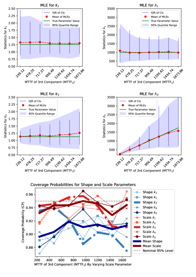
By Equation 5, we see that MTTFj is proportional to the scale parameter , which means when we decrease the scale parameter of a component, we proportionally decrease the MTTF. In this scenario, we start with the well-designed series system described in Table 1, and we will manipulate the MTTF of component 3, MTTF3, by changing its scale parameter, , and observing the effect this has on the MLE. Since the other components had a similar MTTF, we will arbitrarily choose component 1 to represent the other components. The bottom plot shows the coverage probabilities for all parameters.
In Figure 1, we show the effect of changing the scale parameter of component , , but map to MTTF3 to make it more intuitive to reason about. We vary the MTTF of component 3 from to and the other components have their MTTFs fixed at around , as shown in Table 1. We fix the masking probability to (moderate masking), the right-censoring quantile to (moderate censoring), and the sample size to (moderate sample size).
Key Observations
Coverage Probability (CP)
When MTTF of component 3 is much smaller than other components, the CP for is very well calibrated (approximately obtaining the nominal level ) while the CP for other components are around , which is still reasonable. (This is the case even though the width of the CI for is extremely narrow compared to the others). As MTTF3 increases, the CP for decreases, while the CP for the other components increase slightly. The scale parameters are generally well-calibrated for all of the components, except for component 3 when its MTTF is large and it dips down to . Despite the individual differences, the mean of the CPs for shape and scale parameters hardly change.
Dispersion of MLEs
For component 3, as its MTTF decreases, the dispersion of MLEs narrows, indicating more precise estimates. Conversely, dispersion for other components widens. As MTTF of component 3 increases, its dispersion widens while others narrow. This is consistent with the fact that the smaller MTTF of component 3 means that, in this well-designed system at least, it is more likely to be the component cause of failure, and so we have more information about its parameters and are able to estimate them more accurately.
IQR of Bootstrapped CIs
The dark blue vertical lines representing IQR are consistent with the dispersion of MLEs, which is the ideal behavior, and suggests that the BCa confidence intervals are performing well.
Bias of MLEs
For component 3, the bias of MLE for the scale parameter becomes slightly more negatively biased as MTTF3 increases, and the bias of the MLE for the shape parameter becomes slightly more positively biased. The MLE for the shape and scale parameters for component 1 have a very small bias, if any, and are not affected by the MTTF3. The scale parameters are easier to estimate than the shape parameters, and so they are less sensitive to changes in scale than the shape parameters, as we will show in the next scenario.
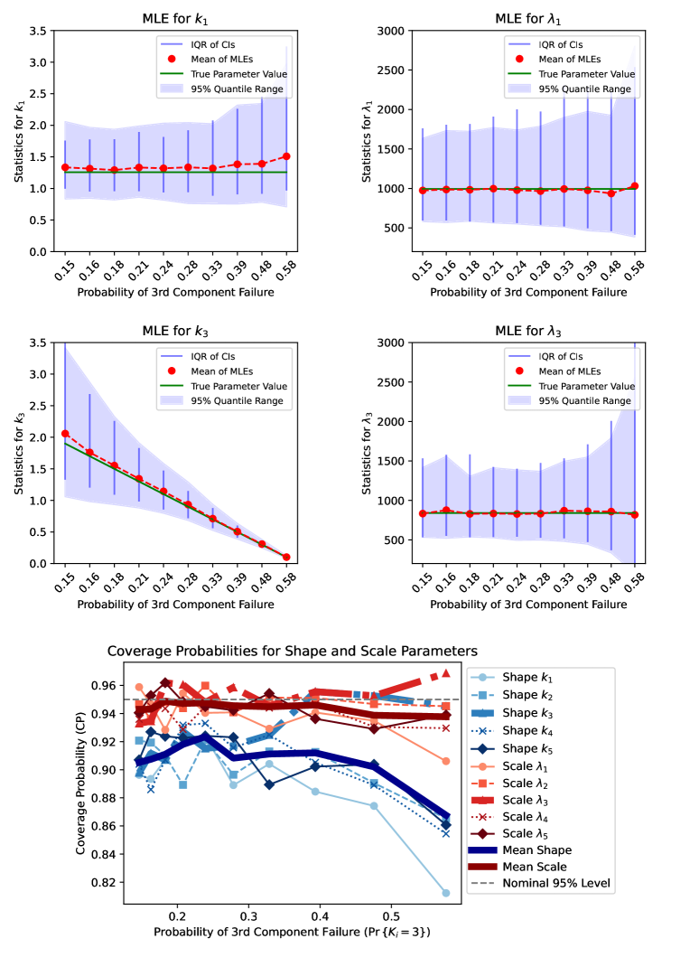
4.3 Scenario: Assessing the Impact of Changing the Shape Parameter of Component 3
The shape parameter determines the failure characteristics. We vary the shape parameter of component 3 from to and observe the effect it has on the MLE. When , this indicates infant mortality, and when , this indicates wear-out failures.
We analyze the effect of component 3’s shape parameter on the MLE and the bootstrapped confidence intervals for the shape and scale parameters of components 1 and 3 (the component we are varying). First, we look at the effect on the scale parameter.
Key Observations
Coverage Probability (CP)
The CP for the scale parameters are well-calibrated and close to the nominal level of for all values of . For the shape parameter of component 3 () in bold orange colors, we see that it is well-calibrated for all values of , but actually may become too large for extreme values of . The CP for the shape parameters of the other components decreases with , dipping below for . At a sample size of , the CP for the shape parameters of the other components is generally not well-calibrated for .
Dispersion of MLEs
The dispersion of the MLE for the shape and scale parameters of component 1, and , is fairly steady but begins to increase rapidly at the extreme values of . This is indicative of having less information about the failure characteristics of component as component begins to dominate the component cause of failure. The dispersion of the shape parameter is initially quite large, indicative of having very little information about the failure characteristics of component 3 since it is unlikely to be the component cause of failure, but its dispersion rapidly decreases as increases and more information is available about component 3’s failure characteristics. In fact, it nearly becomes a point at . The dispersion of the scale parameter of component , , is quite steady and is less spread out than the MLE for , but at extreme values of , it also begins to rapidly increase, suggesting some complex interactions between the shape and scale parameters of component 3.
IQR of Bootstrapped CIs
The CIs precisely track the dispersion of the MLEs, which is the ideal behavior, and suggests that the BCa confidence intervals are performing well.
Bias of MLEs
The MLE for the scale parameters are nearly unbiased and generally seem unaffected by changes in . As increases, the MLE exhibits increasing positive bias for , which corresponds to reduced early-failure behavior for component 1. Conversely, the MLE for shows decreasing positive bias, reflecting higher early-failure rates that are consistent with component 3 dominating as the cause of system failure.
5 Weibull Series Homogeneous Shape Model
The sensitivity analysis in Section 4 demonstrated that while the MLE remains reasonably robust under deviations from a well-designed system, estimator dispersion increases as individual component parameters diverge from the baseline configuration. In this section, we develop a reduced model that assumes homogeneity in the shape parameters of the components, which simplifies analysis and reduces estimator variability.
Here, our focus shifts to a sensitivity analysis aimed at understanding when it is appropriate to use the reduced model that assumes homogeneity in the shape parameters of the components. The reduced model offers interpretability (the series system is itself Weibull) and reduced estimator variability (only parameters instead of ), but it must adequately describe the data.
5.1 Homogeneous Shape Model Definition
The homogeneous shape model (also called the reduced model) assumes that all components share a common shape parameter while retaining individual scale parameters . The parameter vector for the reduced model is
| (15) |
reducing the number of parameters from in the full model to in the reduced model.
Under this assumption, each component has a Weibull lifetime with
| (16) |
A key property of the homogeneous shape model is that the series system lifetime distribution is itself Weibull. We state this precisely as a theorem.
Theorem 5.1 (Weibull Closure for Series Systems).
Let be independent random variables with for . Then the series system lifetime is Weibull-distributed:
| (17) |
Moreover, this closure property is unique to the common-shape constraint: no other single-parameter restriction on the full -parameter model yields a Weibull system lifetime.
Proof.
By Equation (6), the series system reliability function under the common-shape constraint is
where , which is the reliability function of a distribution. For uniqueness, observe that a Weibull system reliability requires the exponent in (6) to factor as for some . This demands for all , which holds if and only if all are equal, since a sum of distinct power functions cannot be a single power function. ∎
This Weibull property of the system lifetime provides several advantages:
-
1.
Analytical tractability: System reliability metrics (MTTF, reliability function, hazard function) have closed-form expressions.
-
2.
Interpretability: The system exhibits a single failure mode characterized by the common shape parameter .
-
3.
Reduced variance: Fewer parameters to estimate results in lower estimator variance, particularly for the shape parameter.
-
4.
Computational efficiency: Optimization is faster with parameters instead of parameters.
However, the reduced model is appropriate only when components genuinely have similar failure characteristics. When component shape parameters differ substantially, forcing homogeneity can lead to poor model fit and biased parameter estimates.
5.2 Model Hierarchy and Motivation
A natural question is: why focus on the homogeneous-shape reduction rather than other simplifications of the full model? Several nested models can be obtained by constraining the parameters of the full model:
| Model | Parameters | Count | System Weibull? | Physical Plausibility |
|---|---|---|---|---|
| Full | No | General | ||
| Common shape | Yes | Same aging, different lifetimes | ||
| Common scale | No | Different aging, same lifetime | ||
| Fully homogeneous | Yes | Identical components | ||
| Exponential | with | Yes | No aging |
The common-shape model occupies a unique position in this hierarchy for three reasons: mathematical, physical, and empirical.
Mathematical: Weibull closure.
By Theorem 5.1, a series system of Weibull components with a common shape parameter is itself Weibull with shape and system scale . This closure property is unique to the common-shape constraint: no other single-parameter restriction on the full model yields a Weibull system lifetime. In particular, setting all scales equal (common-scale model) produces a system reliability function , which is not Weibull when the are heterogeneous. This makes the common-shape model the only single-constraint reduction that preserves the analytical tractability of the Weibull family at the system level.
Physical: same aging mechanism, different lifetimes.
In a well-designed system, components are manufactured to similar quality standards and operate under similar environmental conditions, producing similar aging behavior (shape parameters near 1.1–1.3 in our baseline). However, components differ in size, load capacity, and materials, leading to genuinely different characteristic lifetimes (scale parameters). The common-shape model captures exactly this factorization: shared failure mechanism with component-specific durability. By contrast, the common-scale model would assert that components have similar characteristic lifetimes but fundamentally different failure mechanisms—one exhibiting infant mortality while another exhibits wear-out—which rarely occurs in well-designed systems.
Empirical: the fully homogeneous model is too restrictive.
To assess whether the next simplification beyond common shape is viable, we tested the fully homogeneous model (, for all ) against the full model using the baseline well-designed system. Despite the modest scale CV of 5.4% in our baseline (Table 1), the fully homogeneous model is rejected at rates of 58% (), 89% (), and 99% () at . Component 3’s scale of 840 differs from component 1’s scale of 994 by 18%, and this difference is reliably detected. Scale heterogeneity is real and important even in well-designed systems; only shape homogeneity is a tenable simplification.
Taken together, the common-shape model is the natural “Goldilocks” point in the hierarchy: it is the most parsimonious model that (1) preserves the Weibull property of the system, (2) reflects the physical structure of well-designed systems, and (3) is empirically supported by the data. The remainder of this section investigates where the boundary of this sweet spot lies—how much shape heterogeneity can be present before the common-shape model becomes inadequate.
5.3 Assessing the Appropriateness of the Reduced Model
In order to determine if a reduced model (e.g., Weibull series system in which all of the shape parameters are homogeneous) is appropriate, a hypothesis test may be conducted to determine if there is statistically significant evidence against the null hypothesis that all of the shape parameters are homogeneous. If the test fails to reject , the reduced model is supported; if it rejects , the full model with heterogeneous shapes is preferred.
The likelihood function of the reduced model is related to the likelihood function of the full model. We denote the full model likelihood function by and the reduced model likelihood by . The reduced model is obtained by setting the shape parameter of each component to be the same, i.e., . Thus, the reduced model likelihood function is given by
The same may be done for the score and hessian of the log-likelihood functions.
Given that we employ a well-defined likelihood model, the likelihood ratio test (LRT) is a good choice. The LRT statistic is given by
where is the likelihood of the reduced (null) model evaluated at its MLE given a random sample of masked data and is the likelihood of the full model evaluated at its MLE given the same set of data . Under the null model, the LRT statistic is asymptotically distributed chi-squared with degrees of freedom, where is the number of components in the series system,
If the LRT statistic is greater than the critical value of the chi-squared distribution with degrees of freedom, , where denotes the significance level, then we find the data to be incompatible with the null hypothesis .
5.4 Quantifying Divergence from Homogeneity
To assess how far a system deviates from the homogeneous-shape assumption, we introduce a divergence metric based on the coefficient of variation (CV) of the shape parameters:
| (18) |
A system with has perfectly homogeneous shape parameters, while larger values indicate greater heterogeneity. An alternative metric is the max/min ratio, , which equals 1 for homogeneous systems.
Table 3 shows how varying in our baseline system translates to different divergence levels. The well-designed baseline () has CV and max/min , representing very mild heterogeneity.
| CV (%) | Max/Min | Mean | |
|---|---|---|---|
| 0.25 | 42.2 | 5.03 | 1.01 |
| 0.50 | 29.7 | 2.52 | 1.06 |
| 0.75 | 18.4 | 1.68 | 1.11 |
| 1.00 | 8.3 | 1.26 | 1.16 |
| 1.13 | 4.0 | 1.11 | 1.19 |
| 1.25 | 3.4 | 1.08 | 1.21 |
| 1.50 | 11.0 | 1.29 | 1.26 |
| 2.00 | 26.4 | 1.72 | 1.36 |
| 3.00 | 51.6 | 2.58 | 1.56 |
5.5 Simulation Study: Full Weibull Model vs Reduced (Homogeneous Shape) Model
We aim to assess the appropriateness of the reduced model under varying divergence levels (controlled by ) and sample sizes. We employ a simulation study using the likelihood ratio test (LRT) for this purpose, where the null hypothesis, , assumes homogeneous shape parameters.
We take the well-designed series system described in Table 1, and manipulate the shape parameter of the third component () to cause the components to have different failure characteristics. As shown in Table 3, corresponds to a well-designed series system with CV , while extreme values like or produce systems with CV . We also vary the sample size to assess the impact of sample size on the appropriateness of the reduced model.
Simulation Design.
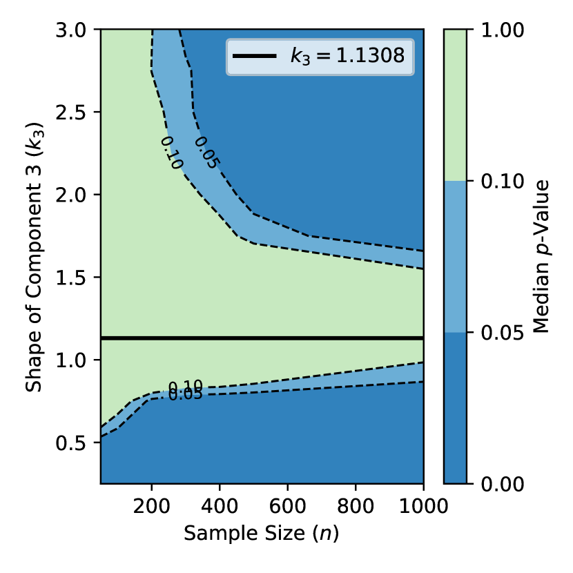
For the contour plot analysis, we varied over 13 values from to (including the baseline value ), and sample sizes over 21 values ranging from to . For the well-designed system analysis (Figure 4), we extended sample sizes up to . Each condition was replicated 1000 times to obtain stable estimates of the -value distribution. The masking probability () and censoring quantile () were held fixed throughout.
Figure 3 provides a contour plot with sample size along the -axis, shape parameter along the -axis, and median -value indicated by color. The contour lines at and represent common significance thresholds. Regions with low -values (dark blue) indicate significant evidence against the reduced model, while regions with high -values (lighter colors) indicate insufficient evidence to reject the reduced model.
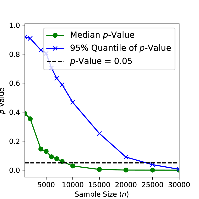
Figure 4 provides a plot of the median -value against the sample size for the well-designed system, where the shape parameter of component 3 is fixed at . The th percentile of the -values is also provided as a more stringent criterion for statistical significance.
Sensitivity to Sample Size ()
-
•
The sample size is an essential aspect of hypothesis testing, as it affects the test’s power, which is the probability of correctly rejecting the null hypothesis when it is false. In the contour plot in Figure 3, as increases, the contours trend lower. This indicates that larger samples result in smaller median -values, implying that the power of the LRT increases with the sample size. However, its power is quite low for small samples, particularly for values of somewhat close to the shape parameters of the other components in the system.
-
•
Recall that in the well-designed series system, . In this case, even very large sample sizes do not produce evidence against the null model, indicating robust compatibility.
-
•
In Figure 4, we fix at and vary the sample size. The median -value only manages to drop below the threshold with sample sizes around . In the more stringent criterion given by the th percentile of the -values, nearly observations are necessary to reject the null hypothesis in of the simulations.
Sensitivity to Divergence from Homogeneity
-
•
In Figure 3, for a given divergence level, increasing the sample size tends to decrease the median -value. Larger samples provide more information about the parameters, which increases the power of the LRT.
-
•
The median -values in the vicinity of the well-designed baseline (, CV ) are high across various sample sizes, indicating that the null model is a good fit for systems with low divergence. As divergence increases (either by decreasing toward 0.25 or increasing toward 3.0), the median -value diminishes rapidly, indicating increasing evidence against the null model. Specifically:
-
–
At CV (), the reduced model remains difficult to reject
-
–
At CV (), modest sample sizes begin to show evidence against the reduced model
-
–
At CV ( or ), even small samples reject the reduced model
-
–
The preceding analysis focused on p-values as a function of divergence and sample size. However, a complete assessment of the LRT requires validation that the test maintains correct Type I error under the null hypothesis and characterization of its power properties. We address these questions in the following extended simulation study.
5.6 Extended Simulation Study: Type I Error and Power Analysis
The previous analysis focused on p-values from the LRT under varying divergence levels. To provide a more complete understanding of LRT behavior, we conducted additional simulations examining: (1) Type I error control under perfect homogeneity, (2) power curves across divergence levels, and (3) the effects of masking probability, censoring, and system complexity on test performance.
5.6.1 Type I Error Validation
A critical validation is whether the LRT maintains correct Type I error when the null hypothesis is true (i.e., when shapes are perfectly homogeneous). Table 4 presents rejection rates at for systems with (all ) across sample sizes from to .
| Sample Size | Rejection Rate | 95% CI | Status |
|---|---|---|---|
| 100 | 0.066 | [0.044, 0.088] | OK |
| 500 | 0.056 | [0.036, 0.076] | OK |
| 1000 | 0.050 | [0.031, 0.069] | OK |
| 5000 | 0.046 | [0.028, 0.064] | OK |
| 10000 | 0.054 | [0.034, 0.074] | OK |
All rejection rates are consistent with the nominal , with 95% confidence intervals containing the nominal level. This confirms that the LRT has correct Type I error control across all sample sizes tested. The asymptotic distribution provides an accurate approximation to the null distribution of the test statistic.
5.6.2 Power Curves by Divergence Level
Figure 5 presents the LRT power (rejection rate) as a function of shape parameter divergence (CV) for different sample sizes. The key insight is that the high rejection rates observed for the baseline well-designed system (CV ) at large sample sizes are not Type I error inflation—they represent the LRT correctly detecting true heterogeneity.
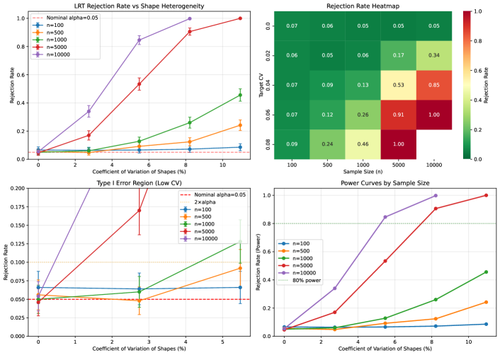
Table 5 summarizes the rejection rates across divergence levels and sample sizes. The results demonstrate that:
-
•
At CV = 0% (perfect homogeneity): Rejection 5% (Type I error controlled)
-
•
At CV = 2.7%: Power is modest ( at , at )
-
•
At CV = 5.5%: Power increases substantially ( at , at )
-
•
At CV : Power exceeds 90% for
| CV (%) | |||||
|---|---|---|---|---|---|
| 0.0 | 0.07 | 0.06 | 0.05 | 0.05 | 0.05 |
| 2.7 | 0.06 | 0.05 | 0.06 | 0.17 | 0.34 |
| 5.5 | 0.07 | 0.09 | 0.13 | 0.53 | 0.85 |
| 8.2 | 0.07 | 0.12 | 0.26 | 0.91 | 1.00 |
| 11.0 | 0.09 | 0.24 | 0.46 | 1.00 | — |
To achieve 80% power to detect heterogeneity, the minimum CV required is approximately:
-
•
: CV
-
•
: CV
This quantifies the practical limits of the LRT for detecting shape heterogeneity.
5.6.3 Factors Affecting LRT Power
We examined how masking probability, censoring level, and system complexity affect LRT performance. These simulations used the baseline well-designed system (CV ), where rejection rates above the nominal 5% indicate power to detect the true (small) heterogeneity.
Effect of Masking Probability.
Figure 6 shows rejection rates as a function of masking probability for different sample sizes. Higher masking reduces information about which component caused each failure, thereby reducing power to detect shape heterogeneity.
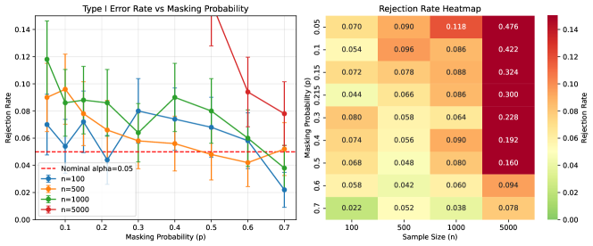
Key observations:
-
•
At , rejection rate drops from 48% at to 8% at
-
•
Higher masking reduces the effective information content, reducing power
-
•
At smaller sample sizes (), rejection rates remain near nominal regardless of masking level
Effect of Censoring Level.
Figure 7 shows rejection rates as a function of censoring quantile . Lower values of correspond to heavier censoring (more observations censored before failure).
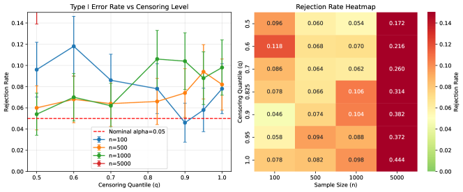
Key observations:
-
•
At , rejection rate increases from 17% at (50% censored) to 44% at (no censoring)
-
•
Censored observations provide only reliability information (system survived to time ), not failure attribution
-
•
Less censoring provides more complete failure information, increasing power
Effect of Number of Components.
Figure 8 shows rejection rates as a function of the number of components in the series system. For each system size, we used shape parameters from the baseline configuration (CV decreasing slightly with more components as shapes regress toward the mean).
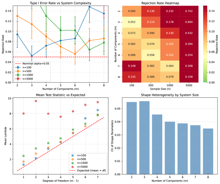
Key observations:
-
•
At , rejection rate decreases from 74% at to 16% at
-
•
The LRT has degrees of freedom, so larger systems have higher critical values
-
•
With more components, failure information is distributed across more parameters, reducing power per parameter
-
•
Smaller systems with similar total CV are easier to distinguish from homogeneous
5.7 Implications and Recommendations
The extended simulation study reveals that the LRT has correct Type I error control and predictable power characteristics. The power of the LRT for well-designed series systems (CV ) is remarkably low, requiring many thousands of observations before the test has sufficient power to reject the null hypothesis. This is not necessarily problematic—it indicates that the reduced model genuinely fits well-designed systems.
Our analysis suggests practical guidelines based on divergence levels:
-
1.
Low divergence (CV ): Use the reduced model confidently. The LRT will not reject it even with very large samples, and it provides the benefits of simplicity, interpretability, and reduced variance.
-
2.
Moderate divergence (CV 10–20%): The choice depends on sample size. For , the reduced model is unlikely to be rejected and may be preferred. For larger samples, consider the full model.
-
3.
High divergence (CV ): Use the full model. Even modest sample sizes will reject the reduced model, indicating genuine heterogeneity that should be captured.
For systems believed to be well-designed, employing the reduced model is supported both statistically and practically due to its simplicity, reduced estimator variability, and analytical tractability. When prior information about component homogeneity is unavailable, engineers should estimate the shape CV from initial data to guide model selection.
5.8 Comparison with Information Criteria
The likelihood ratio test is not the only tool for model selection. The Akaike Information Criterion (AIC) and Bayesian Information Criterion (BIC) are widely used information-theoretic alternatives. We compare these criteria to the LRT using the same fitted log-likelihoods from our simulation study.
For two competing models with log-likelihoods (full, parameters) and (reduced, parameters), the criteria are
| AIC | (19) | |||
| BIC | (20) |
where is the number of parameters and is the sample size. Each criterion selects the full model when its value is lower for the full model than for the reduced model. The key difference lies in the penalty: AIC uses a fixed penalty of , while BIC’s penalty grows with sample size, increasingly favoring parsimonious models.
Figure 9 shows the selection rates for all three criteria as a function of shape parameter divergence (CV). The contrasting calibration properties are immediately apparent.
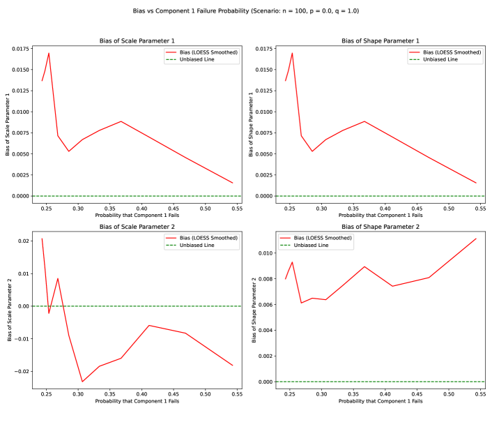
Table 6 presents the Type I error comparison under perfect homogeneity (), where selection of the full model is a false positive.
| Criterion | Selection Rate Range | Behavior |
|---|---|---|
| LRT () | 4.6–6.8% | Well-calibrated |
| AIC | 8.2–12.4% | Liberal ( nominal) |
| BIC | 0–0.2% | Over-conservative |
The LRT maintains rejection rates consistent with the nominal across all sample sizes tested (Table 4). AIC, by contrast, selects the full model at roughly twice the nominal rate under the null hypothesis, with its false positive rate ranging from 8.2% to 12.4%. This liberal behavior is a consequence of AIC’s fixed penalty: the difference in penalty between models () does not grow with sample size, so random fluctuations in the log-likelihood ratio increasingly exceed this threshold as grows. BIC is far more conservative, selecting the full model in at most 0.2% of replications under , because its penalty difference () grows with and rapidly dominates the log-likelihood gain.
The power comparison reveals a complementary tradeoff. At with , the LRT achieves 69% power, AIC selects the full model 78% of the time, and BIC selects it only 3.2% of the time. AIC detects heterogeneity earliest, but at the cost of inflated false positives. BIC’s sample-size-dependent penalty makes it increasingly conservative—nearly never selecting the full model under , but also slow to detect genuine heterogeneity. At larger divergence levels (), all three criteria converge to 100% detection, so the distinction matters primarily in the practically important regime of mild to moderate heterogeneity.
In summary, the LRT provides the best-calibrated Type I error while offering good power, making it the most appropriate criterion for formal hypothesis testing of shape homogeneity. AIC may be useful for exploratory analysis where false positives are less costly than missed heterogeneity. BIC’s conservatism aligns with its known preference for parsimonious models but makes it unsuitable for detecting the subtle shape heterogeneity that characterizes well-designed systems.
6 Conclusion
This paper investigated model selection for reliability estimation in series systems with Weibull component lifetimes, using simulation studies and likelihood ratio tests to determine when a reduced homogeneous-shape model is appropriate.
Model hierarchy.
The common-shape model occupies a unique position among simplifications of the full -parameter Weibull series model. By Theorem 5.1, it is the only single-parameter constraint that renders the series system lifetime itself Weibull, preserving closed-form expressions for all standard reliability metrics. The next simplification—the fully homogeneous model with common shape and scale—is rejected at rates of 58–99% even for our well-designed baseline system, confirming that scale heterogeneity is real and important. The common-shape model thus represents the most parsimonious viable reduction.
Robustness of the reduced model.
The most striking finding of this study is the robustness of the common-shape assumption for well-designed systems. With shape parameter CV below 10%, the LRT cannot reject the reduced model even with sample sizes approaching 30,000—far larger than typically available in practice. This means practitioners can confidently halve the parameter count from to without sacrificing model fit, gaining reduced estimator variance, improved interpretability, and computational efficiency.
Practical decision framework.
Our results support a simple decision framework based on shape parameter divergence:
-
•
CV : Use the reduced model confidently. The LRT will not reject it even with very large samples.
-
•
CV 10–20%: The choice depends on sample size. For , the reduced model is unlikely to be rejected and may be preferred for its lower variance. For larger samples, consider the full model.
-
•
CV : Use the full model. Even modest sample sizes will reject the reduced model, indicating genuine heterogeneity that should be captured.
Comparison with information criteria.
Among the model selection tools evaluated, the LRT provides the best-calibrated Type I error (4.6–6.8% at nominal ) while maintaining good power. AIC selects the full model at roughly twice the nominal rate under the null hypothesis, making it liberal but potentially useful for exploratory analysis. BIC is over-conservative, selecting the full model in at most 0.2% of null replications, which makes it unsuitable for detecting the subtle heterogeneity characteristic of well-designed systems. For formal hypothesis testing of shape homogeneity, the LRT is recommended.
Data quality effects.
Higher masking probabilities and heavier censoring reduce the power of the LRT by diminishing the information available for discriminating between models, but they do not inflate the Type I error rate. The test remains well-calibrated across all masking (–) and censoring (–) conditions tested. This robustness is important for practical applications where data quality cannot always be controlled.
Future directions.
Several extensions merit investigation. First, the common-shape assumption could be tested for non-Weibull component distributions (e.g., log-normal or gamma) where analogous closure properties may or may not hold. Second, optimal experimental design for model selection—determining the sample size, censoring level, and diagnostic effort that maximize discriminatory power—would provide direct guidance for test planning. Third, extending the analysis to parallel and -out-of- system configurations would broaden the applicability of these results to a wider class of reliability problems.
Appendix A Parameter Sensitivity Analysis Tables
This appendix provides detailed tables quantifying the relationships between Weibull parameters and component failure probabilities for a simplified 3-component series system. These tables present illustrative pedagogical examples, not results from the 5-component simulation studies in the main text. The simplified 3-component system allows clear demonstration of the complex, non-linear relationships between shape parameters, scale parameters, mean time to failure (MTTF), and the probability of each component causing system failure. These examples support the theoretical discussions in Section 2 about counterintuitive failure probability patterns.
A.1 Effect of Varying Shape Parameter
Table 7 shows the effect of varying the shape parameter of component 1 () from 0.1 to 1.0 while holding and all scale parameters at .
| MTTF1 | MTTF2 | MTTF3 | System MTTF | ||||
|---|---|---|---|---|---|---|---|
| 0.10 | 0.77 | 0.12 | 0.12 | 10.00 | 2.00 | 2.00 | 0.89 |
| 0.20 | 0.69 | 0.15 | 0.15 | 4.59 | 2.00 | 2.00 | 1.02 |
| 0.30 | 0.64 | 0.18 | 0.18 | 3.32 | 2.00 | 2.00 | 1.10 |
| 0.40 | 0.59 | 0.20 | 0.20 | 2.68 | 2.00 | 2.00 | 1.17 |
| 0.50 | 0.55 | 0.22 | 0.22 | 2.29 | 2.00 | 2.00 | 1.22 |
| 0.60 | 0.52 | 0.24 | 0.24 | 2.03 | 2.00 | 2.00 | 1.27 |
| 0.70 | 0.48 | 0.26 | 0.26 | 1.85 | 2.00 | 2.00 | 1.31 |
| 0.80 | 0.45 | 0.27 | 0.27 | 1.71 | 2.00 | 2.00 | 1.34 |
| 0.90 | 0.42 | 0.29 | 0.29 | 1.61 | 2.00 | 2.00 | 1.38 |
| 1.00 | 0.40 | 0.30 | 0.30 | 1.53 | 2.00 | 2.00 | 1.41 |
Key observations from Table 7:
-
•
As increases from 0.1 to 1.0, the failure probability decreases from 0.77 to 0.40, while and increase proportionally.
-
•
Component 1 has the highest MTTF when (MTTF), yet also has the highest failure probability (). This counter-intuitive result demonstrates that MTTF alone is insufficient for predicting failure probabilities in series systems with heterogeneous shape parameters.
-
•
The shape parameter dominates early hazard behavior. Components with exhibit high infant mortality, making them likely to fail first despite having longer MTTFs than components with .
-
•
System MTTF increases as approaches 1.0, reflecting reduced infant mortality in the overall system.
A.2 Effect of Varying Scale Parameter
Table 8 shows the effect of varying the scale parameter of component 1 () from 1 to 4 while holding all shape parameters at and .
| MTTF1 | MTTF2 | MTTF3 | System MTTF | ||||
|---|---|---|---|---|---|---|---|
| 1.0 | 0.55 | 0.22 | 0.22 | 2.00 | 2.00 | 2.00 | 1.22 |
| 2.0 | 0.35 | 0.32 | 0.32 | 4.00 | 2.00 | 2.00 | 1.72 |
| 3.0 | 0.25 | 0.38 | 0.38 | 6.00 | 2.00 | 2.00 | 1.98 |
| 4.0 | 0.20 | 0.40 | 0.40 | 8.00 | 2.00 | 2.00 | 2.14 |
Key observations from Table 8:
-
•
Unlike the shape parameter, the scale parameter exhibits a more intuitive relationship: as increases, MTTF1 increases proportionally and decreases.
-
•
When shape parameters are homogeneous (), the component with the largest scale parameter has the lowest failure probability, and MTTF is directly proportional to the scale parameter.
-
•
System MTTF increases with , but at a decreasing rate due to the series configuration (weakest link).
-
•
This more linear relationship makes scale parameters easier to estimate than shape parameters, which is consistent with observations in the simulation studies.
A.3 Joint Variation of Shape and Scale Parameters
Table 9 shows the joint effect of varying both and simultaneously, demonstrating the complex interactions between these parameters.
| MTTF1 | MTTF2 | MTTF3 | System MTTF | |||||
|---|---|---|---|---|---|---|---|---|
| 0.25 | 1.0 | 0.64 | 0.18 | 0.18 | 3.63 | 2.00 | 2.00 | 1.10 |
| 0.25 | 2.0 | 0.50 | 0.25 | 0.25 | 7.26 | 2.00 | 2.00 | 1.43 |
| 0.25 | 3.0 | 0.41 | 0.29 | 0.29 | 10.89 | 2.00 | 2.00 | 1.62 |
| 0.50 | 1.0 | 0.55 | 0.22 | 0.22 | 2.00 | 2.00 | 2.00 | 1.22 |
| 0.50 | 2.0 | 0.35 | 0.32 | 0.32 | 4.00 | 2.00 | 2.00 | 1.72 |
| 0.50 | 3.0 | 0.25 | 0.38 | 0.38 | 6.00 | 2.00 | 2.00 | 1.98 |
| 0.75 | 1.0 | 0.48 | 0.26 | 0.26 | 1.40 | 2.00 | 2.00 | 1.31 |
| 0.75 | 2.0 | 0.25 | 0.38 | 0.38 | 2.80 | 2.00 | 2.00 | 1.98 |
| 0.75 | 3.0 | 0.16 | 0.42 | 0.42 | 4.19 | 2.00 | 2.00 | 2.32 |
Key observations from Table 9:
-
•
For a fixed shape parameter , increasing decreases (component 1 becomes less likely to fail first).
-
•
For a fixed scale parameter , increasing also decreases , but the mechanism is different: higher reduces infant mortality.
-
•
The joint effects are multiplicative rather than additive. A component with low shape () and high scale () still has MTTF = 10.89 and , demonstrating the dominance of early hazard behavior in series systems.
-
•
To minimize a component’s failure probability, both increasing its scale parameter and increasing its shape parameter toward 1.0 are effective strategies, but they work through different mechanisms.
A.4 Implications for Model Selection and Estimation
These tables quantitatively demonstrate several key principles that inform the simulation studies and model selection analyses in the main text:
-
1.
MTTF is insufficient: Component failure probabilities depend on the entire hazard function shape, not just the mean. Systems with heterogeneous shape parameters require careful analysis beyond MTTF comparisons.
-
2.
Shape parameter complexity: The non-linear relationship between shape parameters and failure probabilities explains why shape parameters are harder to estimate and exhibit greater bias than scale parameters.
-
3.
Information availability: Components with high failure probabilities provide more data for estimation. When is small, parameter estimates for component will have high variance regardless of sample size.
-
4.
Model selection criteria: The reduced model (homogeneous shapes) is appropriate when shape parameters are already similar, as failure probabilities become more predictable from MTTF alone. When shape parameters diverge substantially, the full model is necessary to capture the complex failure probability structure.
Appendix B Ideal Case Analysis: No Masking or Censoring
This appendix examines MLE behavior under ideal conditions—complete data with no masking () and no censoring (). This “best case” scenario establishes baseline estimator performance when the true failed component is always known and all systems are observed until failure. Understanding this baseline helps separate inherent estimation challenges from complications introduced by masked and censored data.
B.1 Simulation Setup
We simulated a 2-component series system with parameters similar to our main study but simplified for clearer visualization. The failure probability of component 1, , was varied from 0 to 0.55 by adjusting the shape parameter while holding other parameters fixed. For each configuration, 1000 replications were performed with observations per replication.
B.2 Results
Figure 10 shows LOESS-smoothed estimates of shape and scale parameters as a function of the true failure probability .

B.3 Key Observations
-
1.
Bias persists even in ideal conditions: Shape parameter estimates exhibit bias even without masking or censoring. This reflects the inherent difficulty of estimating Weibull shape parameters from limited samples, particularly for components with low failure probabilities.
-
2.
Information asymmetry: Components with higher failure probabilities ( near 0.5) provide more information for estimation, resulting in lower bias and variance. Components that rarely cause system failure yield less precise estimates regardless of data quality.
-
3.
Scale parameters are more stable: Consistent with findings in the main text, scale parameter estimates show less sensitivity to failure probability than shape parameters. This robustness persists even in the ideal case.
-
4.
Baseline for masked/censored comparisons: The bias patterns observed here represent the “floor” of estimation difficulty. Any additional bias in the main simulation studies (with , ) can be attributed to information loss from masking and censoring.
B.4 Implications
The ideal case analysis confirms that MLE challenges in series systems are not solely due to data complications. Even with perfect information about which component failed and complete observation of all failures, shape parameter estimation remains difficult for components with low failure probabilities. This underscores the importance of the model selection guidance in the main text: when component shapes are genuinely similar, the reduced model’s pooling of information across components can improve estimation by effectively increasing the sample size for the common shape parameter.
References
- [1] (1995) A limited memory algorithm for bound constrained optimization. SIAM Journal on Scientific Computing 16 (5), pp. 1190–1208. Cited by: §3.4, 6th item.
- [2] (1987) Better bootstrap confidence intervals. Journal of the American Statistical Association 82 (397), pp. 171–185. Cited by: 7th item.
- [3] (1989-10) An iterative approach for estimating component reliability from masked system life data. Quality and Reliability Engineering International 5 (4), pp. 257–261. External Links: Document, Link Cited by: §1.1.
- [4] (1991-09) Estimating system and component reliabilities under partial information on cause of failure. Journal of Statistical Planning and Inference 29, pp. 75–85. External Links: Document, Link Cited by: §1.
- [5] (2013-01) Estimating component reliabilities from incomplete system failure data. Annual Reliability and Maintainability Symposium (RAMS), pp. 1–6. External Links: Document, ISBN 9781467347112; 1467347116; 9781467347099; 1467347094; 9781467347105; 1467347108 Cited by: §1.1.
- [6] (1996-06) Bayes estimation of component-reliability from masked system-life data. IEEE Transactions on Reliability vol. 45 iss. 2 45 (2), pp. 233–237. External Links: Document Cited by: §1.1.
- [7] (2001-10) Reliability estimations of components from masked system life data. Reliability Engineering & System Safety 74 (1), pp. 107–113. External Links: Document Cited by: §1.1.
- [8] (2004-03) Parameter estimations in linear failure rate model using masked data. Applied Mathematics and Computation 151 (1), pp. 233–249. External Links: Document, Link Cited by: §1.1.
- [9] (2005-06) Estimation of component failure probability from masked binomial system testing data. Reliability Engineering & System Safety vol. 88 iss. 3 88 (3), pp. 301–309. External Links: Document Cited by: §1.1.
- [10] (2007-02) Estimation of exponential component reliability from uncertain life data in series and parallel systems. Reliability Engineering & System Safety 92 (2), pp. 223–230. External Links: Document, Link Cited by: §1.1.
- [11] (2023) Reliability estimation in series systems: maximum likelihood techniques for right-censored and masked failure data. Note: [Online; accessed 2023-09-30] External Links: Link Cited by: §1.1, item 2, item 6, §3.4, §3.
- [12] (1988) Maximum likelihood analysis of component reliability using masked system life-test data. IEEE Transactions on Reliability 37 (5), pp. 550–555. External Links: Document, Link Cited by: §1.1.
- [13] (1993) Exact maximum likelihood estimation using masked system data. IEEE Transactions on Reliability 42 (4), pp. 631–635. External Links: Document, Link Cited by: §1.1.
- [14] (1996-06) Weibull component reliability-prediction in the presence of masked data. IEEE Transactions on Reliability 45 (2), pp. 229–232. External Links: Document, ISSN 0018-9529,1558-1721, Link Cited by: §1.1.