Relaxed Candidate Set Models for Masked Data in Series Systems

Alex Towell
lex@metafunctor.com

(February 4, 2026)

Abstract

We develop likelihood-based inference methods for series systems with masked failure data when the traditional conditions governing candidate set formation are relaxed. While existing methods require that masking be non-informative (Condition C2) and parameter-independent (Condition C3), practical diagnostic systems often violate these assumptions. We derive the likelihood under various relaxation scenarios, establish identifiability conditions, and compare Fisher information under standard versus relaxed models. Our analysis reveals that informative masking, when properly modeled, can paradoxically improve estimation efficiency by providing additional information about the failed component. Simulation studies quantify the bias from incorrectly assuming standard conditions when masking is informative (C2 violation) or parameter-dependent (C3 violation), and demonstrate that the framework extends to Weibull series systems. We implement these methods in the mdrelax R package.

Keywords: Series systems, masked data, reliability estimation, informative masking, candidate sets, Fisher information, maximum likelihood estimation

1 Introduction

Estimating the reliability of individual components in a series system presents a fundamental challenge in reliability engineering: system-level failure data is observable, but component-level failure causes are often masked. When a series system fails, diagnostic procedures may identify only a candidate set of components that could have caused the failure, rather than pinpointing the exact failed component [7]. This masking, combined with right-censoring of system lifetimes, complicates statistical inference about component reliability parameters.

Prior work on masked data in series systems has established a tractable likelihood framework under three conditions [6]:

•

C1: The failed component is always contained in the candidate set.
•

C2: Masking is non-informative—conditional on the failure time and candidate set, each component in the candidate set is equally likely to have failed.
•

C3: The masking mechanism does not depend on the system parameters $\bm{\theta}$ .

Under these conditions, the likelihood has a simple closed form that enables efficient maximum likelihood estimation (MLE). However, practical diagnostic systems may violate C2 and C3:

•

Experienced technicians may preferentially include components that “seem likely” to have failed based on failure time characteristics, violating C2.
•

Diagnostic algorithms based on reliability rankings may systematically favor certain components, with the ranking depending on the true parameters, violating C3.

This paper develops the theoretical and computational framework for likelihood-based inference when C2 and/or C3 are relaxed while maintaining C1. Our contributions are:

1.

General likelihood framework. We derive the likelihood under C1 alone, showing how informative and parameter-dependent masking modify the standard likelihood structure (Section 3).
2.

Practical masking models. We introduce the rank-based informative masking model and the Bernoulli candidate set model with KL-divergence constraints, which provide interpretable parameterizations of non-standard masking (Section 3).
3.

Identifiability analysis. We establish conditions under which parameters remain identifiable when standard conditions fail, including the surprising result that informative masking can improve identifiability in certain cases (Section 4).
4.

Efficiency comparison. We derive the Fisher information matrix under relaxed conditions for exponential series systems, enabling precise comparison of estimation efficiency (Section 4).
5.

Simulation studies. We quantify the bias from incorrectly assuming C2 when masking is informative, and demonstrate the improved estimation achievable when the masking structure is properly modeled (Section 5).

The remainder of this paper is organized as follows. Section 2 reviews series systems, masked data, and the standard C1-C2-C3 likelihood. Section 3 develops the likelihood under relaxed conditions. Section 4 analyzes identifiability and Fisher information. Section 5 presents simulation studies. Section 6 discusses practical implications, and Section 7 concludes.

2 Background

2.1 Series System Model

Consider a series system composed of $m$ components. The lifetime of the $i$ -th system is

T_{i}=\min\{T_{i1},T_{i2},\ldots,T_{im}\},

(1)

where $T_{ij}$ denotes the lifetime of the $j$ -th component in the $i$ -th system. Component lifetimes are assumed independent with parametric distributions indexed by $\bm{\theta}_{j}$ ; the full parameter vector is $\bm{\theta}=(\bm{\theta}_{1},\ldots,\bm{\theta}_{m})\in\bm{\Omega}$ .

Definition 2.1 (Component Distribution Functions).

For component $j$ with parameter $\bm{\theta}_{j}$ :

$\displaystyle R_{j}(t;\bm{\theta}_{j})$	$\displaystyle=\mathrm{Pr}\{T_{ij}>t\}$	$\displaystyle\text{(reliability function)},$	(2)
$\displaystyle f_{j}(t;\bm{\theta}_{j})$	$\displaystyle=-\frac{d}{dt}R_{j}(t;\bm{\theta}_{j})$	$\displaystyle\text{(density function)},$	(3)
$\displaystyle h_{j}(t;\bm{\theta}_{j})$	$\displaystyle=\frac{f_{j}(t;\bm{\theta}_{j})}{R_{j}(t;\bm{\theta}_{j})}$	$\displaystyle\text{(hazard function)}.$	(4)

For the series system, these functions combine as follows:

Theorem 2.2 (Series System Distribution Functions).

The series system has:

$\displaystyle R_{T_{i}}(t;\bm{\theta})$	$\displaystyle=\prod_{j=1}^{m}R_{j}(t;\bm{\theta}_{j}),$	(5)
$\displaystyle h_{T_{i}}(t;\bm{\theta})$	$\displaystyle=\sum_{j=1}^{m}h_{j}(t;\bm{\theta}_{j}),$	(6)
$\displaystyle f_{T_{i}}(t;\bm{\theta})$	$\displaystyle=h_{T_{i}}(t;\bm{\theta})\cdot R_{T_{i}}(t;\bm{\theta}).$	(7)

The proof follows from the independence of component lifetimes and standard arguments [6].

2.2 Component Cause of Failure

Let $K_{i}\in\{1,\ldots,m\}$ denote the index of the component that caused system $i$ to fail. Since the system fails when the first component fails, $K_{i}=\arg\min_{j}T_{ij}$ .

Theorem 2.3 (Joint Distribution of $(T_{i},K_{i})$ ).

The joint distribution of system lifetime and component cause of failure is:

f_{T_{i},K_{i}}(t,k;\bm{\theta})=h_{k}(t;\bm{\theta}_{k})\prod_{\ell=1}^{m}R_{% \ell}(t;\bm{\theta}_{\ell}).

(8)

The proof follows from the definition of the series system minimum and the independence of component lifetimes; see [6] for details.

Corollary 2.4 (Conditional Failure Probability).

Given that the system failed at time $t$ , the probability that component $j$ caused the failure is:

\mathrm{Pr}\{K_{i}=j\mid T_{i}=t\}=\frac{h_{j}(t;\bm{\theta}_{j})}{\sum_{\ell=% 1}^{m}h_{\ell}(t;\bm{\theta}_{\ell})}.

(9)

This follows immediately from Theorem 2.3 and Bayes’ theorem; see [6].

This probability plays a central role in masked data analysis, as it represents the “true” probability that each component failed, which the masking mechanism partially obscures.

2.3 Masked Data Structure

Definition 2.5 (Observed Data).

For each system $i$ , we observe:

•

$S_{i}=\min\{T_{i},\tau_{i}\}$ : Right-censored system lifetime,
•

$\delta_{i}=\mathbf{1}_{T_{i}\leq\tau_{i}}$ : Event indicator ( $1$ if failure observed, $0$ if censored),
•

$C_{i}\subseteq\{1,\ldots,m\}$ : Candidate set (only observed when $\delta_{i}=1$ ).

The latent (unobserved) variables are:

•

$K_{i}\in\{1,\ldots,m\}$ : Index of failed component,
•

$(T_{i1},\ldots,T_{im})$ : Component failure times.

2.4 Traditional Conditions C1, C2, C3

The existing literature [7, 8, 4] establishes tractable likelihood-based inference under three conditions:

Condition 1 (C1: Failed Component in Candidate Set).

The candidate set always contains the failed component:

\mathrm{Pr}\{K_{i}\in C_{i}\}=1.

(10)

Condition 2 (C2: Non-Informative Masking).

Given the failure time and that the failed component is in a candidate set $c$ , the probability of observing $c$ does not depend on which component in $c$ failed:

\mathrm{Pr}\{C_{i}=c\mid T_{i}=t,K_{i}=j\}=\mathrm{Pr}\{C_{i}=c\mid T_{i}=t,K_% {i}=j^{\prime}\}

(11)

for all $j,j^{\prime}\in c$ .

Condition 3 (C3: Parameter-Independent Masking).

The masking probabilities do not depend on the system parameters:

\mathrm{Pr}\{C_{i}=c\mid T_{i}=t,K_{i}=j\}=\beta_{i}(c,t,j),

(12)

where $\beta_{i}$ does not depend on $\bm{\theta}$ .

2.5 Likelihood Under C1, C2, C3

Under all three conditions, the likelihood admits a tractable form:

Theorem 2.6 (Likelihood Under C1-C2-C3).

Under Conditions C1, C2, and C3, the likelihood contribution from an uncensored observation $(s_{i},c_{i})$ is proportional to:

L_{i}(\bm{\theta})\propto\prod_{\ell=1}^{m}R_{\ell}(s_{i};\bm{\theta}_{\ell})% \cdot\sum_{k\in c_{i}}h_{k}(s_{i};\bm{\theta}_{k}).

(13)

For a censored observation with lifetime $s_{i}$ :

L_{i}(\bm{\theta})=\prod_{\ell=1}^{m}R_{\ell}(s_{i};\bm{\theta}_{\ell}).

(14)

The proof proceeds by summing over $K_{i}$ and applying C1, C2, C3 in sequence to factor and then eliminate the masking probability; see [6] for the full derivation.

The complete log-likelihood for $n$ independent systems is:

\ell(\bm{\theta})=\sum_{i=1}^{n}\left[\sum_{j=1}^{m}\log R_{j}(s_{i};\bm{% \theta}_{j})+\delta_{i}\log\left(\sum_{k\in c_{i}}h_{k}(s_{i};\bm{\theta}_{k})% \right)\right].

(15)

2.6 Related Work

The masked data problem in series systems was introduced by Usher and Hodgson [7], who developed MLE methods for exponential components. Usher et al. [8] extended this to Weibull components with exact maximum likelihood. Guo et al. [4] (Guo et al.) provided simulation studies validating the approach under various masking scenarios.

The informative censoring literature in survival analysis [5, 3] addresses related issues where the censoring mechanism depends on covariates or outcomes. However, the candidate set structure in masked data creates a distinct problem not fully addressed by standard informative censoring methods.

The competing risks framework [1] provides another perspective, viewing component failures as competing causes of system failure. However, standard competing risks methods assume the cause is observed, whereas masked data only provides partial information through candidate sets.

Our work extends the C1-C2-C3 framework by explicitly modeling departures from C2 and C3, providing both theoretical analysis and practical estimation methods.

3 Relaxed Candidate Set Models

We now develop the likelihood framework when conditions C2 and/or C3 are relaxed while maintaining C1. The key insight is that the general likelihood structure remains tractable—it simply requires modeling the masking mechanism explicitly rather than treating it as a nuisance.

3.1 General Likelihood Under C1

Theorem 3.1 (Likelihood Under C1 Alone).

Under Condition C1 alone, the likelihood contribution from an uncensored observation $(s_{i},c_{i})$ is:

L_{i}(\bm{\theta})=\prod_{\ell=1}^{m}R_{\ell}(s_{i};\bm{\theta}_{\ell})\cdot% \sum_{k\in c_{i}}h_{k}(s_{i};\bm{\theta}_{k})\cdot\mathrm{Pr}_{\bm{\theta}}\{C% _{i}=c_{i}\mid T_{i}=s_{i},K_{i}=k\}.

(16)

Proof.

Under C1, $\mathrm{Pr}_{\bm{\theta}}\{C_{i}=c\mid T_{i}=t,K_{i}=k\}=0$ when $k\notin c$ . Therefore, summing over $K_{i}$ :

	$\displaystyle f_{T_{i},C_{i}}(t,c;\bm{\theta})$	$\displaystyle=\sum_{k=1}^{m}h_{k}(t;\bm{\theta}_{k})\prod_{\ell=1}^{m}R_{\ell}% (t;\bm{\theta}_{\ell})\cdot\mathrm{Pr}_{\bm{\theta}}\{C_{i}=c\mid T_{i}=t,K_{i% }=k\}$		(17)
		$\displaystyle=\prod_{\ell=1}^{m}R_{\ell}(t;\bm{\theta}_{\ell})\cdot\sum_{k\in c% }h_{k}(t;\bm{\theta}_{k})\mathrm{Pr}_{\bm{\theta}}\{C_{i}=c\mid T_{i}=t,K_{i}=% k\}.\qed$		(18)

Remark 3.1 (Comparison with C1-C2-C3).

Under C2, the masking probability can be factored out of the sum since it is constant over $k\in c$ . Under C3, it can be dropped since it does not depend on $\bm{\theta}$ . When either condition fails, the masking probabilities remain inside the sum and may depend on both $k$ and $\bm{\theta}$ , fundamentally changing the inference problem.

3.2 Relaxing C2: Informative Masking

When C2 is violated but C1 and C3 hold, the masking probability $\mathrm{Pr}\{C_{i}=c\mid T_{i}=t,K_{i}=k\}$ can vary with $k\in c$ .

Definition 3.2 (Informative Masking).

Let $\pi_{kc}(t)=\mathrm{Pr}\{C_{i}=c\mid T_{i}=t,K_{i}=k\}$ for $k\in c$ . The masking is informative if $\pi_{kc}(t)$ varies with $k$ .

Theorem 3.3 (Likelihood Under C1 and C3 (Relaxed C2)).

Under C1 and C3, the likelihood contribution is:

L_{i}(\bm{\theta})=\prod_{\ell=1}^{m}R_{\ell}(s_{i};\bm{\theta}_{\ell})\cdot% \sum_{k\in c_{i}}h_{k}(s_{i};\bm{\theta}_{k})\cdot\pi_{k,c_{i}}(s_{i}),

(19)

where $\pi_{k,c}(t)$ does not depend on $\bm{\theta}$ (by C3).

When $\pi_{kc}(t)$ is known, the likelihood remains tractable. The masking probabilities act as weights on the hazard contributions from each candidate.

3.2.1 Rank-Based Informative Masking

A practical model for informative masking assigns inclusion probabilities based on component failure ranks rather than absolute times.

Definition 3.4 (Rank-Based Masking).

Let $r_{k}(\mathbf{t})\in\{1,\ldots,m\}$ denote the rank of component $k$ ’s failure time among $(t_{1},\ldots,t_{m})$ , where rank 1 corresponds to the earliest failure (the actual failed component).

The probability that component $j$ is in the candidate set is:

q_{j}=\begin{cases}1&\text{if }r_{j}=1\text{ (failed component)},\\ \beta\exp(-\alpha(r_{j}-2))&\text{if }r_{j}\geq 2,\end{cases}

(20)

where $\alpha\geq 0$ controls the decay rate and $\beta\in[0,1]$ is the maximum inclusion probability for non-failed components.

Remark 3.2 (Limiting Behavior).

•

As $\alpha\to 0$ : All non-failed components have probability $\beta$ (uninformative within the non-failed set).
•

As $\alpha\to\infty$ : Only the failed component and rank-2 component have non-zero probabilities.

This model captures the intuition that components failing “nearly at the same time” as the actual failure are more likely to be included in the candidate set.

3.2.2 General Bernoulli Candidate Set Model

The most general Bernoulli model for candidate set formation allows the inclusion probability of each component to depend on which component actually failed.

Definition 3.5 (General Bernoulli Model).

Let $p_{j}(k)$ denote the probability that component $j$ is included in the candidate set given that component $k$ failed:

p_{j}(k)=\mathrm{Pr}\{j\in C_{i}\mid K_{i}=k\}.

(21)

Under C1, we require $p_{j}(j)=1$ for all $j$ . These probabilities can be organized into an $m\times m$ matrix $\mathbf{P}$ :

\mathbf{P}=\begin{pmatrix}1&p_{1}(2)&\cdots&p_{1}(m)\\ p_{2}(1)&1&\cdots&p_{2}(m)\\ \vdots&\vdots&\ddots&\vdots\\ p_{m}(1)&p_{m}(2)&\cdots&1\end{pmatrix},

(22)

where the $(j,k)$ entry is $p_{j}(k)=\mathrm{Pr}\{j\in C\mid K=k\}$ .

Remark 3.3 (Time-Independence Assumption).

The most general Bernoulli model would allow $p_{j}(k,t)$ to depend on the failure time $t$ as well as the failed component $k$ . We simplify by assuming time-independence: $p_{j}(k,t)=p_{j}(k)$ for all $t$ . This is a reasonable assumption when the masking mechanism depends on which component failed but not on when the failure occurred. Time-dependent models are left to future work.

Remark 3.4 (Condition C2 in Terms of $\mathbf{P}$ ).

Condition C2 holds if and only if each row of $\mathbf{P}$ has constant off-diagonal entries, i.e., $p_{j}(k)=p_{j}$ for all $k\neq j$ . Relaxing C2 allows each column to have different values, meaning the masking mechanism “knows” something about which component failed.

The probability of observing candidate set $c$ given that component $k$ failed is:

\pi_{k}(c)=\mathrm{Pr}\{C=c\mid K=k\}=\mathbf{1}_{k\in c}\prod_{j\in c% \setminus\{k\}}p_{j}(k)\prod_{j\notin c}(1-p_{j}(k)).

(23)

Theorem 3.6 (Likelihood Under General Bernoulli Model).

Under the general Bernoulli model with C1 (and C3), the likelihood contribution from an uncensored observation $(s_{i},c_{i})$ is:

L_{i}(\bm{\theta},\mathbf{P})=\prod_{\ell=1}^{m}R_{\ell}(s_{i};\bm{\theta}_{% \ell})\cdot\sum_{k\in c_{i}}h_{k}(s_{i};\bm{\theta}_{k})\cdot\pi_{k}(c_{i}),

(24)

where $\pi_{k}(c_{i})$ is given by (23).

Remark 3.5 (Nuisance Parameters).

The off-diagonal entries of $\mathbf{P}$ constitute $m(m-1)$ nuisance parameters that must be estimated alongside the $m$ rate parameters $\bm{\theta}$ (for exponential components). The total parameter count is $m^{2}$ .

3.2.3 Simplified Bernoulli Model (C2 Satisfied)

A special case assumes the inclusion probabilities do not depend on $k$ :

Definition 3.7 (Simplified Bernoulli Model).

Each component $j$ is included in the candidate set independently with probability $q_{j}$ , subject to C1 (failed component always included):

p_{j}(k)=\begin{cases}1&\text{if }j=k,\\ q_{j}&\text{if }j\neq k.\end{cases}

(25)

This model satisfies C2 since the masking probability does not depend on which component $k\in c$ actually failed.

Under this simplified model, the probability of observing candidate set $c$ given $(T_{i}=t,K_{i}=k)$ is:

\mathrm{Pr}\{C_{i}=c\mid T_{i}=t,K_{i}=k\}=\mathbf{1}_{k\in c}\prod_{j\in c% \setminus\{k\}}q_{j}\prod_{j\notin c}(1-q_{j}).

(26)

Proposition 3.8 (Likelihood Under Simplified Bernoulli Model).

Under the simplified Bernoulli model with C1, C2 and known probabilities $(q_{1},\ldots,q_{m})$ , the likelihood contribution is:

L_{i}(\bm{\theta})=\prod_{\ell=1}^{m}R_{\ell}(s_{i};\bm{\theta}_{\ell})\cdot% \sum_{k\in c_{i}}h_{k}(s_{i};\bm{\theta}_{k})w_{k}(c_{i}),

(27)

where

w_{k}(c)=\prod_{j\in c\setminus\{k\}}q_{j}\prod_{j\notin c}(1-q_{j})

(28)

is the probability of observing $c$ given that $k$ failed. Note that $w_{k}(c)$ is the same for all $k\in c$ (by C2), so it factors out and the likelihood reduces to the C1-C2-C3 form up to a constant.

3.2.4 KL-Divergence Constrained Models

To systematically study deviations from the standard C1-C2-C3 model, we can parameterize informative masking by its distance from the baseline:

Definition 3.9 (KL-Divergence from Baseline).

Let $P=(p,\ldots,p,1,p,\ldots,p)$ denote the baseline Bernoulli model satisfying C1-C2-C3, where the failed component has probability 1 and all others have probability $p$ .

For a given target KL-divergence $d\geq 0$ , we seek a masking probability vector $Q=(q_{1},\ldots,q_{m})$ satisfying:

1.

$q_{k}=1$ for the failed component (C1),
2.

$\mathrm{KL}(P\|Q)\approx d$ ,
3.

$\sum_{j}q_{j}=\sum_{j}p_{j}$ (same expected candidate set size).

When $d=0$ , we recover $Q=P$ (the C1-C2-C3 model). As $d$ increases, $Q$ becomes more informative about which component failed. This provides a controlled framework for studying the effects of departures from C2.

3.3 Relaxing C3: Parameter-Dependent Masking

When C3 is violated, the masking probability $\mathrm{Pr}_{\bm{\theta}}\{C_{i}=c\mid T_{i}=t,K_{i}=k\}$ depends on $\bm{\theta}$ .

Theorem 3.10 (Likelihood Under C1 and C2 (Relaxed C3)).

Under C1 and C2, the likelihood contribution is:

L_{i}(\bm{\theta})=\pi_{c_{i}}(s_{i};\bm{\theta})\cdot\prod_{\ell=1}^{m}R_{% \ell}(s_{i};\bm{\theta}_{\ell})\cdot\sum_{k\in c_{i}}h_{k}(s_{i};\bm{\theta}_{% k}),

(29)

where $\pi_{c}(t;\bm{\theta})=\mathrm{Pr}_{\bm{\theta}}\{C_{i}=c\mid T_{i}=t,K_{i}\in c\}$ is the (common) masking probability for any $k\in c$ , now depending on $\bm{\theta}$ .

Proof.

By C2, we can factor out the masking probability since it is constant over $k\in c$ :

	$\displaystyle f_{T_{i},C_{i}}(t,c;\bm{\theta})$	$\displaystyle=\prod_{\ell=1}^{m}R_{\ell}(t;\bm{\theta}_{\ell})\sum_{k\in c}h_{% k}(t;\bm{\theta}_{k})\mathrm{Pr}_{\bm{\theta}}\{C_{i}=c\mid T_{i}=t,K_{i}=k\}$		(30)
		$\displaystyle=\pi_{c}(t;\bm{\theta})\prod_{\ell=1}^{m}R_{\ell}(t;\bm{\theta}_{% \ell})\sum_{k\in c}h_{k}(t;\bm{\theta}_{k}).\qed$		(31)

Remark 3.6 (Nuisance Parameters).

When $\pi_{c}(t;\bm{\theta})$ has a known functional form, it contributes to the likelihood and affects the MLE. If the form is unknown, additional modeling assumptions or profile likelihood approaches may be needed.

3.3.1 Failure-Probability-Weighted Masking

A natural way for masking to depend on $\bm{\theta}$ is through the conditional failure probabilities:

Definition 3.11 (Failure-Probability-Weighted Masking).

The probability that component $j$ is in the candidate set depends on its posterior failure probability:

\mathrm{Pr}_{\bm{\theta}}\{j\in C_{i}\mid T_{i}=t\}=g\left(\frac{h_{j}(t;\bm{% \theta}_{j})}{\sum_{\ell=1}^{m}h_{\ell}(t;\bm{\theta}_{\ell})}\right)

(32)

for some function $g:[0,1]\to[0,1]$ with $g(x)\to 1$ as $x\to 1$ .

This models diagnosticians who are more likely to include components with higher failure probabilities given the observed failure time. The function $g$ controls the sensitivity of masking to these probabilities.

3.3.2 Power-Weighted Hazard Model

A particularly tractable form uses hazard rates raised to a power $\alpha$ :

Definition 3.12 (Power-Weighted Masking).

The inclusion probability for component $j$ is proportional to its hazard rate raised to power $\alpha\geq 0$ :

\mathrm{Pr}_{\bm{\theta}}\{j\in C_{i}\mid T_{i}=t\}=\frac{h_{j}(t;\bm{\theta}_% {j})^{\alpha}}{\sum_{\ell=1}^{m}h_{\ell}(t;\bm{\theta}_{\ell})^{\alpha}}.

(33)

Remark 3.7 (Limiting Cases).

•

$\alpha=0$ : Uniform distribution over all components (uninformative).
•

$\alpha=1$ : Inclusion proportional to hazard (posterior failure probability).
•

$\alpha\to\infty$ : Assigns probability 1 to the component with highest hazard rate (maximally informative).

For exponential components with rates $\theta_{1},\ldots,\theta_{m}$ , the hazards are constant, so the inclusion probability for component $j$ becomes $\theta_{j}^{\alpha}/\sum_{\ell}\theta_{\ell}^{\alpha}$ , independent of $t$ .

Remark 3.8 (Relaxing C1).

Under power-weighted masking with large $\alpha$ , the true failed component has high posterior probability of being included even without enforcing C1. This suggests that for “maximally informative” masking models, the strict requirement that $K\in C$ (C1) may be relaxed to a softer constraint.

Remark 3.9 (Model Misspecification Risk).

Parameter-dependent masking models like (33) represent strong assumptions about the data-generating process. If the assumed masking mechanism is incorrect, the resulting MLEs may be severely biased.

For example, if data are generated under the simple Bernoulli model (C1-C2-C3) but analyzed under the power-weighted model with $\alpha>0$ , the estimator will attribute variation in candidate sets to hazard rate differences rather than random masking, leading to biased rate estimates.

This contrasts with the conservative C1-C2-C3 approach: when C2 and C3 hold, the masking mechanism is non-informative and can be “integrated out,” making inference robust to the specific masking probabilities. When relaxing these conditions, the analyst trades robustness for potential efficiency gains, but only when the assumed masking model is correct.

3.4 The General Case: Both C2 and C3 Relaxed

When both C2 and C3 are relaxed, the likelihood takes the fully general form from Theorem 3.1:

L_{i}(\bm{\theta})=\prod_{\ell=1}^{m}R_{\ell}(s_{i};\bm{\theta}_{\ell})\cdot% \sum_{k\in c_{i}}h_{k}(s_{i};\bm{\theta}_{k})\cdot\pi_{k,c_{i}}(s_{i};\bm{% \theta}).

(34)

Estimation in this general case requires either:

1.

A fully specified parametric model for $\pi_{k,c}(t;\bm{\theta})$ , or
2.

Sensitivity analysis over plausible masking mechanisms, or
3.

Nonparametric or semiparametric approaches that avoid specifying the masking mechanism.

In practice, the most common scenario is relaxed C2 with C3 maintained (informative but parameter-independent masking), which we focus on in the simulation studies.

3.5 Simulation Evidence: Robustness of Relaxed C2

We conducted simulation studies to evaluate the practical implications of model choice when C2 may or may not hold. The key question: What is the cost of using the more flexible relaxed-C2 model when C2 actually holds?

3.5.1 Simulation Design

We consider an exponential series system with $m=2$ components and true parameters $\theta_{1}=1$ , $\theta_{2}=2$ . Each scenario uses $n=400$ observations with right-censoring time $\tau=5$ (moderate censoring).

Scenario 1:: Data generated under C1-C2-C3 ( $p=0.3$ ), analyzed with C1-C2-C3 model. (Baseline)
Scenario 2b:: Data generated under C1-C2-C3 ( $p=0.3$ ), analyzed with relaxed-C2 model using known $\mathbf{P}$ .
Scenario 3:: Data generated under relaxed C2 ( $\mathbf{P}$ asymmetric), analyzed with C1-C2-C3 model. (Misspecified)
Scenario 4b:: Data generated under relaxed C2 ( $\mathbf{P}$ asymmetric), analyzed with relaxed-C2 model using known $\mathbf{P}$ .

For the asymmetric $\mathbf{P}$ matrix, we use $p_{1}(2)=0.8$ (component 1 very likely included when component 2 fails) and $p_{2}(1)=0.1$ (component 2 unlikely when component 1 fails).

3.5.2 Results

Scenario	Model	Rel. Bias $\theta_{1}$	Rel. Bias $\theta_{2}$	RMSE $\theta_{1}$	RMSE $\theta_{2}$
1 (C2 holds)	C1-C2-C3	0.7%	1.6%	9.7%	7.2%
2b (C2 holds)	Relaxed C2 (known $\mathbf{P}$ )	0.7%	1.6%	9.6%	7.2%
3 (C2 violated)	C1-C2-C3	109%	$-$ 53%	110%	54%
4b (C2 violated)	Relaxed C2 (known $\mathbf{P}$ )	2.2%	0.0%	10.7%	7.2%

Table 1: Simulation results comparing model robustness. Relative bias and RMSE as percentage of true parameter value. Based on 50 replications.

3.5.3 Interpretation

1.

Relaxed C2 is safe when C2 holds (Scenarios 1 vs. 2b): Using the more flexible relaxed-C2 model on data that satisfies C2 incurs essentially no efficiency penalty. Both bias and RMSE are virtually identical.
2.

Misspecification is catastrophic (Scenario 3): Fitting the C1-C2-C3 model when C2 is violated produces severe bias—over 100% for $\theta_{1}$ and $-53\%$ for $\theta_{2}$ . The model misattributes informative masking to component failure rates.
3.

Correct model recovers parameters (Scenario 4b): When the relaxed-C2 model is used with the correct $\mathbf{P}$ , estimates are nearly unbiased with reasonable variance.

Remark 3.10 (Practical Implications).

These results support a conservative modeling strategy: when the masking mechanism is uncertain, use the relaxed-C2 model with an estimated or hypothesized $\mathbf{P}$ matrix. If C2 actually holds, little is lost. If C2 is violated, severe bias is avoided.

However, jointly estimating $\bm{\theta}$ and $\mathbf{P}$ from data alone poses identifiability challenges. In practice, $\mathbf{P}$ should be either: (i) estimated from auxiliary data or expert knowledge, (ii) constrained to a lower-dimensional structure, or (iii) subjected to sensitivity analysis.

3.5.4 Identifiability of Joint Estimation

Additional simulations reveal that the difficulty with joint estimation of $\bm{\theta}$ and $\mathbf{P}$ is not a finite-sample problem. Even with $n=2000$ observations, the joint MLE exhibits persistent bias:

Estimation Method	$\hat{\theta}_{1}$	$\hat{\theta}_{2}$
Joint ( $\bm{\theta}$ , $\mathbf{P}$ )	1.62	1.44
Known $\mathbf{P}$	0.97	2.08
True values	1.00	2.00

The joint estimator consistently converges to $\hat{\theta}\approx(1.6,1.4)$ with $\hat{P}_{21}\approx 0.45$ (true: 0.10), regardless of sample size. This indicates fundamental non-identifiability: different combinations of $(\bm{\theta},\mathbf{P})$ yield similar likelihoods.

Notably, the total hazard $\sum_{j}\theta_{j}$ remains well-identified ( $\hat{\Sigma}\theta=3.01$ vs. true 3.00), but individual components are confounded with the off-diagonal elements of $\mathbf{P}$ .

Remark 3.11 (Implications for Practice).

This non-identifiability result has important practical implications:

1.

If $\mathbf{P}$ can be estimated from auxiliary information (expert knowledge, pilot studies, or the masking process itself), the relaxed-C2 model provides excellent estimates.
2.

If $\mathbf{P}$ is completely unknown, the analyst faces a choice: (a) assume C2 holds and use the simpler model (risking bias if C2 is violated), or (b) impose structural constraints on $\mathbf{P}$ (e.g., symmetry, sparsity) to achieve identifiability.
3.

Sensitivity analysis over plausible $\mathbf{P}$ matrices may reveal how conclusions depend on the assumed masking mechanism.

4 Identifiability and Fisher Information

We now analyze identifiability conditions and derive the Fisher information matrix under relaxed conditions, focusing on exponential series systems for tractability.

4.1 Identifiability Under C1-C2-C3

Definition 4.1 (Identifiability).

A parameter $\bm{\theta}$ is identifiable if for any $\bm{\theta},\bm{\theta}^{\prime}\in\bm{\Omega}$ with $\bm{\theta}\neq\bm{\theta}^{\prime}$ , there exists some data configuration $D$ such that

L(\bm{\theta};D)\neq L(\bm{\theta}^{\prime};D).

(35)

Theorem 4.2 (Identifiability Under C1-C2-C3).

Under C1, C2, and C3, the parameter $\bm{\theta}$ is identifiable if and only if the following condition holds: For each pair of components $j\neq j^{\prime}$ , there exists at least one observed candidate set $c$ such that exactly one of $j\in c$ or $j^{\prime}\in c$ holds (i.e., the components do not always co-occur in candidate sets).

Proof.

The log-likelihood contribution from an uncensored observation is:

\ell_{i}(\bm{\theta})=\sum_{\ell=1}^{m}\log R_{\ell}(s_{i};\bm{\theta}_{\ell})% +\log\left(\sum_{k\in c_{i}}h_{k}(s_{i};\bm{\theta}_{k})\right).

(36)

Sufficiency: If components $j$ and $j^{\prime}$ appear in different candidate sets, then information about $h_{j}$ can be obtained from observations where $j\in c_{i}$ but $j^{\prime}\notin c_{i}$ , and vice versa. Combined with the survival term (which depends on all parameters), this provides sufficient variation to identify individual parameters.

Necessity: If components $j$ and $j^{\prime}$ always co-occur in every candidate set, the hazard sum always contains $h_{j}+h_{j^{\prime}}$ as an inseparable unit. The survival term provides information only about $\sum_{\ell}\lambda_{\ell}$ . Thus, any reparametrization preserving both $h_{j}+h_{j^{\prime}}$ and $\sum_{\ell}h_{\ell}$ yields the same likelihood, demonstrating non-identifiability. ∎

4.2 Block Non-Identifiability

A particularly important case arises when components form blocks that always appear together:

Theorem 4.3 (Block Non-Identifiability).

Suppose components are partitioned into blocks $B_{1},\ldots,B_{r}$ such that for every observed candidate set $c_{i}$ :

(i)

For each block $B_{\ell}$ : either $B_{\ell}\subseteq c_{i}$ or $B_{\ell}\cap c_{i}=\emptyset$ , and
(ii)

If the failed component $k\in B_{\ell}$ , then $B_{\ell}\subseteq c_{i}$ .

Then for exponential components with rates $(\lambda_{1},\ldots,\lambda_{m})$ , only the block sums $\Lambda_{\ell}=\sum_{j\in B_{\ell}}\lambda_{j}$ are identifiable.

Proof.

Under the exponential model with constant hazards, the likelihood becomes:

L(\bm{\theta})\propto\prod_{i:\delta_{i}=1}\exp\left(-s_{i}\sum_{j=1}^{m}% \lambda_{j}\right)\sum_{k\in c_{i}}\lambda_{k}.

(37)

The survival term depends only on $\sum_{j=1}^{m}\lambda_{j}$ . For the hazard sum, under the block structure, each candidate set $c_{i}$ is a union of complete blocks. Thus:

\sum_{k\in c_{i}}\lambda_{k}=\sum_{\ell:B_{\ell}\subseteq c_{i}}\Lambda_{\ell}.

(38)

Any reparametrization that preserves $(\Lambda_{1},\ldots,\Lambda_{r})$ yields the same likelihood, hence individual $\lambda_{j}$ within blocks are not identifiable. ∎

Example 4.1 (Three-Component Block Model).

Consider a 3-component system where the diagnostic tool can only distinguish:

•

Components 1 and 2 share a circuit board (block $B_{1}=\{1,2\}$ ),
•

Component 3 is separate (block $B_{2}=\{3\}$ ).

Candidate sets are either $\{1,2\}$ , $\{3\}$ , or $\{1,2,3\}$ . The MLE satisfies:

	$\displaystyle\hat{\lambda}_{1}+\hat{\lambda}_{2}$	$\displaystyle=\lambda_{1}+\lambda_{2},$		(39)
	$\displaystyle\hat{\lambda}_{3}$	$\displaystyle=\lambda_{3},$		(40)

but individual $\hat{\lambda}_{1},\hat{\lambda}_{2}$ are not unique.

4.3 Improved Identifiability with Informative Masking

Surprisingly, relaxing C2 can improve identifiability:

Theorem 4.4 (Improved Identifiability with Informative Masking).

Under C1 and C3 with known informative masking probabilities $\pi_{kc}(t)$ , identifiability can be improved relative to the C1-C2-C3 case. Specifically, if components $k$ and $k^{\prime}$ always co-occur in candidate sets (violating the identifiability condition of Theorem 4.2), they become identifiable if there exists a candidate set $c$ with $k,k^{\prime}\in c$ such that $\pi_{kc}(t)\neq\pi_{k^{\prime}c}(t)$ for some $t>0$ .

Proof.

Under C1-C2-C3 with non-informative masking, if components $k$ and $k^{\prime}$ always co-occur, the hazard sum contains only the unweighted sum $h_{k}+h_{k^{\prime}}$ , making individual hazards non-identifiable.

Under informative masking with known weights $\pi_{kc}$ , the likelihood contribution becomes:

L_{i}(\bm{\theta})=R(s_{i};\bm{\theta})\sum_{j\in c_{i}}h_{j}(s_{i};\bm{\theta% }_{j})\pi_{j,c_{i}}(s_{i}).

(41)

The hazard sum now involves the weighted combination $h_{k}\pi_{kc}+h_{k^{\prime}}\pi_{k^{\prime}c}$ . If $\pi_{kc}\neq\pi_{k^{\prime}c}$ , this provides one equation involving $h_{k}$ and $h_{k^{\prime}}$ with unequal coefficients.

Combined with the survival term (which contributes $h_{k}+h_{k^{\prime}}$ through the system hazard), we have two linearly independent equations:

	$\displaystyle\pi_{kc}h_{k}+\pi_{k^{\prime}c}h_{k^{\prime}}$	$\displaystyle=A_{1}\quad\text{(from hazard sum)},$		(42)
	$\displaystyle h_{k}+h_{k^{\prime}}$	$\displaystyle=A_{2}\quad\text{(from survival term)}.$		(43)

When $\pi_{kc}\neq\pi_{k^{\prime}c}$ , this system has a unique solution, establishing identifiability of individual hazards. ∎

Remark 4.1.

Informative masking can paradoxically help estimation when the masking structure is known, because it provides additional information about which component likely failed.

4.4 Fisher Information for Exponential Series Systems

We now derive closed-form expressions for the Fisher information matrix, specializing to exponential components.

4.4.1 Exponential Series Model

For exponential components with rates $\bm{\lambda}=(\lambda_{1},\ldots,\lambda_{m})$ :

$\displaystyle R_{j}(t;\lambda_{j})$	$\displaystyle=e^{-\lambda_{j}t},$	(44)
$\displaystyle h_{j}(t;\lambda_{j})$	$\displaystyle=\lambda_{j},$	(45)
$\displaystyle R_{T_{i}}(t;\bm{\lambda})$	$\displaystyle=e^{-\Lambda t},\quad\text{where }\Lambda=\sum_{j=1}^{m}\lambda_{% j}.$	(46)

4.4.2 Fisher Information Under C1-C2-C3

Theorem 4.5 (FIM Under C1-C2-C3).

For the exponential series system under C1, C2, C3, the observed Fisher information matrix has elements:

\mathcal{I}_{jk}(\bm{\lambda})=\sum_{i:\delta_{i}=1}\frac{\mathbf{1}_{j\in c_{% i}}\mathbf{1}_{k\in c_{i}}}{\left(\sum_{\ell\in c_{i}}\lambda_{\ell}\right)^{2% }}.

(47)

Proof.

The log-likelihood for an uncensored observation $i$ is:

\ell_{i}(\bm{\lambda})=-s_{i}\Lambda+\log\left(\sum_{k\in c_{i}}\lambda_{k}% \right).

(48)

The first derivatives (score) are:

\frac{\partial\ell_{i}}{\partial\lambda_{j}}=-s_{i}+\frac{\mathbf{1}_{j\in c_{% i}}}{\sum_{k\in c_{i}}\lambda_{k}}.

(49)

The second derivatives are:

\frac{\partial^{2}\ell_{i}}{\partial\lambda_{j}\partial\lambda_{k}}=-\frac{% \mathbf{1}_{j\in c_{i}}\mathbf{1}_{k\in c_{i}}}{\left(\sum_{\ell\in c_{i}}% \lambda_{\ell}\right)^{2}}.

(50)

The observed FIM is the negative Hessian, giving the result. ∎

Remark 4.2.

The FIM depends on the candidate sets but not on the failure times (for exponential components). This reflects the memoryless property of the exponential distribution.

4.4.3 Fisher Information Under Relaxed C2

Theorem 4.6 (FIM Under Informative Masking).

Under C1, C3, and informative masking with known weights $\pi_{kc}$ , the observed Fisher information matrix for exponential components is:

\mathcal{I}_{jk}(\bm{\lambda})=\sum_{i:\delta_{i}=1}\frac{\pi_{j,c_{i}}\pi_{k,% c_{i}}}{\left(\sum_{\ell\in c_{i}}\lambda_{\ell}\pi_{\ell,c_{i}}\right)^{2}}% \mathbf{1}_{j\in c_{i}}\mathbf{1}_{k\in c_{i}}.

(51)

Proof.

The log-likelihood contribution is:

\ell_{i}(\bm{\lambda})=-s_{i}\Lambda+\log\left(\sum_{k\in c_{i}}\lambda_{k}\pi% _{k,c_{i}}\right).

(52)

The score is:

\frac{\partial\ell_{i}}{\partial\lambda_{j}}=-s_{i}+\frac{\pi_{j,c_{i}}\mathbf% {1}_{j\in c_{i}}}{\sum_{k\in c_{i}}\lambda_{k}\pi_{k,c_{i}}}.

(53)

The Hessian is:

\frac{\partial^{2}\ell_{i}}{\partial\lambda_{j}\partial\lambda_{k}}=-\frac{\pi% _{j,c_{i}}\pi_{k,c_{i}}\mathbf{1}_{j\in c_{i}}\mathbf{1}_{k\in c_{i}}}{\left(% \sum_{\ell\in c_{i}}\lambda_{\ell}\pi_{\ell,c_{i}}\right)^{2}}.\qed

(54)

4.5 Efficiency Comparison

Theorem 4.7 (Relative Efficiency).

Let $\mathcal{I}^{(\text{C123})}$ and $\mathcal{I}^{(\text{C13})}$ denote the Fisher information matrices under C1-C2-C3 and C1-C3 (informative masking) respectively. Then:

(a)

If $\pi_{kc}=1/|c|$ for all $k\in c$ (uniform weighting), then $\mathcal{I}^{(\text{C13})}=\mathcal{I}^{(\text{C123})}$ .
(b)

If masking is highly informative (concentrating weight on one component), $\mathcal{I}^{(\text{C13})}$ can exceed $\mathcal{I}^{(\text{C123})}$ for that component’s parameter.

Proof.

(a) Under C1-C2-C3 (non-informative masking), the FIM element is:

\mathcal{I}_{jk}^{(\text{C123})}=\sum_{i:\delta_{i}=1}\frac{\mathbf{1}_{j\in c% _{i}}\mathbf{1}_{k\in c_{i}}}{\left(\sum_{\ell\in c_{i}}\lambda_{\ell}\right)^% {2}}.

(55)

Under C1-C3 with uniform weights $\pi_{\ell c}=1/|c|$ for all $\ell\in c$ :

$\displaystyle\mathcal{I}_{jk}^{(\text{C13})}$	$\displaystyle=\sum_{i:\delta_{i}=1}\frac{(1/\|c_{i}\|)^{2}\mathbf{1}_{j\in c_{i}% }\mathbf{1}_{k\in c_{i}}}{\left(\sum_{\ell\in c_{i}}\lambda_{\ell}(1/\|c_{i}\|)% \right)^{2}}$	(56)
	$\displaystyle=\sum_{i:\delta_{i}=1}\frac{(1/\|c_{i}\|^{2})\mathbf{1}_{j\in c_{i}% }\mathbf{1}_{k\in c_{i}}}{(1/\|c_{i}\|)^{2}\left(\sum_{\ell\in c_{i}}\lambda_{% \ell}\right)^{2}}$	(57)
	$\displaystyle=\sum_{i:\delta_{i}=1}\frac{\mathbf{1}_{j\in c_{i}}\mathbf{1}_{k% \in c_{i}}}{\left(\sum_{\ell\in c_{i}}\lambda_{\ell}\right)^{2}}=\mathcal{I}_{% jk}^{(\text{C123})}.$	(58)

(b) Suppose $\pi_{kc}=1$ for component $k$ and $\pi_{k^{\prime}c}=0$ for all $k^{\prime}\neq k$ in $c$ . Then:

\mathcal{I}_{kk}^{(\text{C13})}=\sum_{i:\delta_{i}=1,k\in c_{i}}\frac{1}{% \lambda_{k}^{2}}.

(59)

This concentrates all information on $\lambda_{k}$ , which can exceed $\mathcal{I}_{kk}^{(\text{C123})}$ when $|c_{i}|>1$ since the denominator under C1-C2-C3 is $(\sum_{\ell\in c_{i}}\lambda_{\ell})^{2}>\lambda_{k}^{2}$ . ∎

Remark 4.3 (Practical Implications).

Informative masking can either help or hurt estimation:

•

Helps when the masking structure is known and aligned with what we want to estimate.
•

Hurts if masking is informative but we incorrectly assume C2 (non-informative), leading to model misspecification bias.

4.6 Estimation Under Model Misspecification

Theorem 4.8 (Bias from C2 Misspecification).

Suppose the true model is C1-C3 with informative masking $\pi_{kc}(t)$ , but estimation is performed assuming C1-C2-C3 (non-informative masking). The resulting MLE $\hat{\bm{\theta}}$ is generally biased, with bias depending on the correlation between $\pi_{kc}$ and the hazard ratios $h_{k}(t;\bm{\theta}_{k})/\sum_{\ell\in c}h_{\ell}(t;\bm{\theta}_{\ell})$ .

Proof.

The score under the assumed (wrong) C1-C2-C3 model is:

\frac{\partial\ell_{i}^{\text{wrong}}}{\partial\lambda_{j}}=-s_{i}+\frac{% \mathbf{1}_{j\in c_{i}}}{\sum_{k\in c_{i}}\lambda_{k}}.

(60)

The true score under C1-C3 (informative masking) is:

\frac{\partial\ell_{i}^{\text{true}}}{\partial\lambda_{j}}=-s_{i}+\frac{\pi_{j% ,c_{i}}\mathbf{1}_{j\in c_{i}}}{\sum_{k\in c_{i}}\lambda_{k}\pi_{k,c_{i}}}.

(61)

At the true parameter $\bm{\theta}^{*}$ , the true score has expectation zero: $\mathbb{E}[\partial\ell_{i}^{\text{true}}/\partial\lambda_{j}]=0$ .

The misspecified score has expectation:

\displaystyle\mathbb{E}\left[\frac{\partial\ell_{i}^{\text{wrong}}}{\partial% \lambda_{j}}\right]

\displaystyle=-\mathbb{E}[s_{i}]+\mathbb{E}\left[\frac{\mathbf{1}_{j\in c_{i}}% }{\sum_{k\in c_{i}}\lambda_{k}^{*}}\right].

(62)

This differs from zero when the masking weights $\pi_{kc}$ are correlated with the hazard ratios. Specifically, define the “effective” weight $w_{j}=\mathbb{E}[\mathbf{1}_{j\in c}/\sum_{k\in c}\lambda_{k}^{*}]$ under the true model. The MLE under the wrong model solves $\mathbb{E}[\partial\ell^{\text{wrong}}/\partial\lambda_{j}]=0$ , yielding $\hat{\lambda}_{j}$ that satisfies:

\hat{\lambda}_{j}=\frac{\mathbb{E}[\mathbf{1}_{j\in c_{i}}]}{\mathbb{E}[\sum_{% k\in c_{i}}\lambda_{k}^{*}\cdot s_{i}/\sum_{k\in c_{i}}\lambda_{k}^{*}]}.

(63)

When $\pi_{jc}>\pi_{kc}$ for components with larger $\lambda_{j}^{*}$ , the misspecified model overestimates components that are more likely to be in candidate sets, producing systematic bias. ∎

Theorem 4.9 (Bias from C3 Misspecification).

Suppose the true model has parameter-dependent masking (C3 violated) with $\pi_{c}(t;\bm{\theta})=\mathrm{Pr}_{\bm{\theta}}\{C_{i}=c\mid T_{i}=t,K_{i}\in c\}$ , but estimation is performed assuming C1-C2-C3 (ignoring the $\bm{\theta}$ -dependence). The resulting MLE $\hat{\bm{\theta}}$ is generally biased, unless the masking probability $\pi_{c}(t;\bm{\theta})$ is locally constant in $\bm{\theta}$ near the true parameter value.

Proof.

Under the true model (relaxed C3), the log-likelihood contribution is:

\ell_{i}^{\text{true}}(\bm{\theta})=\sum_{j=1}^{m}\log R_{j}(s_{i};\bm{\theta}% _{j})+\delta_{i}\left[\log\left(\sum_{k\in c_{i}}h_{k}(s_{i};\bm{\theta}_{k})% \right)+\log\pi_{c_{i}}(s_{i};\bm{\theta})\right].

(64)

The misspecified model drops the masking term:

\ell_{i}^{\text{wrong}}(\bm{\theta})=\sum_{j=1}^{m}\log R_{j}(s_{i};\bm{\theta% }_{j})+\delta_{i}\log\left(\sum_{k\in c_{i}}h_{k}(s_{i};\bm{\theta}_{k})\right).

(65)

The misspecified score omits $\partial\log\pi_{c_{i}}/\partial\bm{\theta}_{j}$ , which is non-zero when masking depends on $\bm{\theta}$ . Setting the wrong score to zero yields a pseudo-true parameter $\bm{\theta}^{\dagger}$ satisfying:

\mathbb{E}\left[\frac{\partial\ell_{i}^{\text{wrong}}}{\partial\bm{\theta}_{j}% }\bigg{|}_{\bm{\theta}=\bm{\theta}^{\dagger}}\right]=0,

(66)

which differs from $\bm{\theta}^{*}$ unless $\mathbb{E}[\partial\log\pi_{c_{i}}/\partial\bm{\theta}_{j}]=0$ at $\bm{\theta}^{*}$ . ∎

These results motivate the simulation studies in Section 5, which quantify the bias under both C2 and C3 misspecification scenarios.

5 Simulation Studies

We present simulation studies to (1) validate MLE performance under the C1-C2-C3 Bernoulli masking model, (2) quantify the bias from incorrectly assuming C2 when masking is informative, and (3) investigate identifiability issues arising from correlated candidate sets.

5.1 Experimental Design

5.1.1 System Configuration

We consider exponential series systems with $m=3$ components and true rate parameters:

\bm{\lambda}^{*}=(\lambda_{1}^{*},\lambda_{2}^{*},\lambda_{3}^{*})=(1.0,1.5,2.% 0).

(67)

These values represent a system where component 3 has the highest failure rate (and thus contributes most to system failures), while component 1 is most reliable.

5.1.2 Data Generation

For each simulation replicate:

1.

Generate component failure times $T_{ij}\sim\text{Exp}(\lambda_{j}^{*})$ for $i=1,\ldots,n$ and $j=1,\ldots,m$ .
2.

Compute system failure times $T_{i}=\min_{j}T_{ij}$ and identify failed components $K_{i}=\arg\min_{j}T_{ij}$ .
3.

Apply right-censoring at time $\tau$ (chosen to achieve approximately 20% censoring) to obtain observed lifetimes $S_{i}=\min(T_{i},\tau)$ and indicators $\delta_{i}$ .
4.

Generate candidate sets using the specified masking model.

5.1.3 Masking Models

We examine three masking scenarios:

1.

C1-C2-C3 (Baseline): Bernoulli model with $p=0.3$ for all non-failed components.
2.

Informative masking (Rank-based): Masking probabilities depend on component failure time ranks, parameterized by informativeness parameter $\alpha\in\{0,1,2,5,10\}$ .
3.

Correlated candidate sets: Candidate set indicators have correlation $\rho\in\{0,0.1,0.3,0.5,0.6,0.8,0.9\}$ .

5.1.4 Performance Metrics

We evaluate:

•

Bias: $\text{Bias}(\hat{\lambda}_{j})=\mathbb{E}[\hat{\lambda}_{j}]-\lambda_{j}^{*}$
•

Root mean squared error (RMSE): $\text{RMSE}(\hat{\lambda}_{j})=\sqrt{\mathbb{E}[(\hat{\lambda}_{j}-\lambda_{j}% ^{*})^{2}]}$
•

Coverage probability: Proportion of 95% confidence intervals containing $\lambda_{j}^{*}$
•

RMSE ratio: $\text{RMSE}_{\text{misspec}}/\text{RMSE}_{\text{correct}}$

5.2 Study 1: MLE Performance Under Bernoulli Masking

We first validate MLE performance under the correctly specified C1-C2-C3 Bernoulli masking model across sample sizes $n\in\{50,100,200\}$ with $B=200$ Monte Carlo replicates.

5.2.1 Results

Table 2 presents the estimation results.

Table 2: Maximum Likelihood Estimation Performance by Sample Size

$n$	Parameter	Bias	RMSE	Coverage	Mean CI Width
50	$\lambda_{1}$	0.017	0.477	0.920	1.727
	$\lambda_{2}$	0.007	0.511	0.935	1.952
	$\lambda_{3}$	0.085	0.557	0.945	2.197
100	$\lambda_{1}$	0.016	0.318	0.935	1.175
	$\lambda_{2}$	0.055	0.390	0.935	1.385
	$\lambda_{3}$	$-0.037$	0.366	0.950	1.519
200	$\lambda_{1}$	$-0.005$	0.201	0.935	0.825
	$\lambda_{2}$	0.008	0.262	0.965	0.965
	$\lambda_{3}$	$-0.033$	0.258	0.955	1.066

Notes. Results based on 200 Monte Carlo replications. True parameters: $\lambda_{1}=1.0$ , $\lambda_{2}=1.5$ , $\lambda_{3}=2.0$ . Bernoulli masking with $p=0.3$ , censoring proportion $\approx 20\%$ .

Refer to caption — Figure 1: RMSE of MLE by sample size. All three component rate parameters show decreasing RMSE as sample size increases, consistent with $\sqrt{n}$ -convergence.

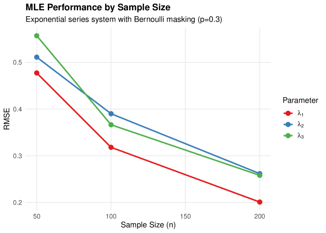
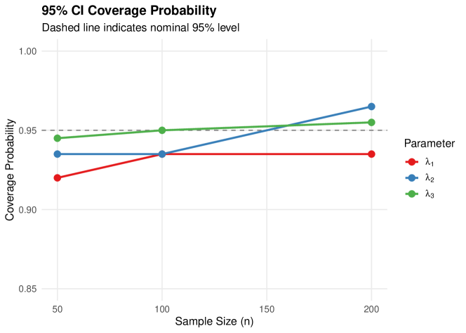
Key findings from Study 1:

1.

Consistency: Bias is small relative to RMSE at all sample sizes, indicating approximate unbiasedness.
2.

Convergence: RMSE decreases from approximately 0.5 at $n=50$ to 0.2–0.3 at $n=200$ , consistent with $\sqrt{n}$ -rate convergence.
3.

Coverage: 95% CI coverage ranges from 92.0% to 96.5%, close to the nominal level, validating the Fisher information-based standard errors.
4.

Component effects: Components with higher true rates ( $\lambda_{3}=2.0$ ) have slightly larger absolute RMSE but similar relative performance.

5.3 Study 2: Misspecification Bias Analysis

We quantify the bias from incorrectly assuming C1-C2-C3 when masking is actually informative. Data is generated with rank-based informative masking (informativeness parameter $\alpha$ ), then analyzed using both the correct model and the misspecified C2 model.

5.3.1 Results

Table 3 compares bias under correct versus misspecified models.

Table 3: Bias Comparison: Correct vs Misspecified Model

$\alpha$	Parameter	Bias (Correct)	Bias (Misspec.)	RMSE Ratio
0	$\lambda_{1}$	$-0.129$	$-0.001$	1.019
	$\lambda_{2}$	0.027	0.024	1.090
	$\lambda_{3}$	0.105	$-0.020$	1.013
1	$\lambda_{1}$	$-0.136$	$-0.095$	0.999
	$\lambda_{2}$	$-0.009$	$-0.004$	1.031
	$\lambda_{3}$	0.192	0.146	0.944
5	$\lambda_{1}$	$-0.129$	$-0.127$	1.002
	$\lambda_{2}$	$-0.005$	0.010	1.031
	$\lambda_{3}$	0.147	0.130	0.988
10	$\lambda_{1}$	$-0.153$	$-0.152$	1.022
	$\lambda_{2}$	0.000	0.002	0.993
	$\lambda_{3}$	0.183	0.178	1.008

Notes. $\alpha=0$ corresponds to non-informative masking (C2 satisfied). As $\alpha$ increases, masking becomes more informative. RMSE Ratio = RMSE(Misspecified) / RMSE(Correct); values $>1$ indicate efficiency loss.

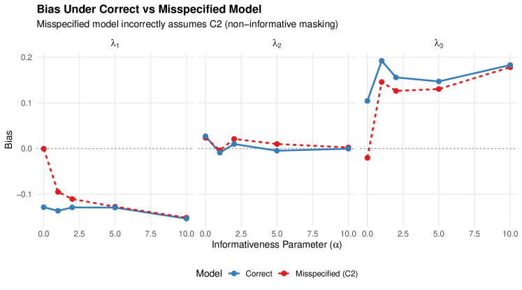
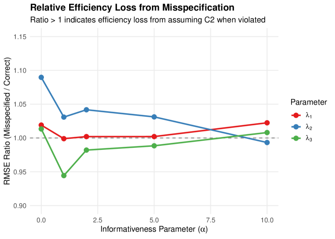
Key findings from Study 2:

1.

Moderate robustness: The RMSE ratio stays between 0.94 and 1.09 across all informativeness levels, indicating that misspecifying the masking model produces at most 9% efficiency loss.
2.

Bias similarity: Surprisingly, bias under the misspecified model closely tracks bias under the correct model, suggesting the C2 assumption is more robust than theoretical arguments might suggest.
3.

Parameter-specific effects: Component 3 ( $\lambda_{3}$ ) shows consistently positive bias under both models, likely due to its higher failure rate making it more frequently the true cause of failure.

5.4 Study 3: Identifiability and Candidate Set Correlation

We investigate how correlation between candidate set indicators affects identifiability by examining the Fisher Information Matrix (FIM) eigenvalues.

5.4.1 Results

Table 4 presents FIM analysis by correlation level.

Table 4: Fisher Information Matrix Analysis by Candidate Set Correlation

$\rho$	Smallest Eigenvalue	Condition Number
0.0	12.23	2.18
0.1	12.93	2.12
0.3	14.17	2.01
0.5	15.00	1.97
0.6	15.12	1.91
0.8	14.33	2.01
0.9	13.88	2.04

Notes. $\rho$ measures correlation between candidate set indicators. As $\rho\to 1$ , components always co-occur in candidate sets, theoretically leading to non-identifiability.

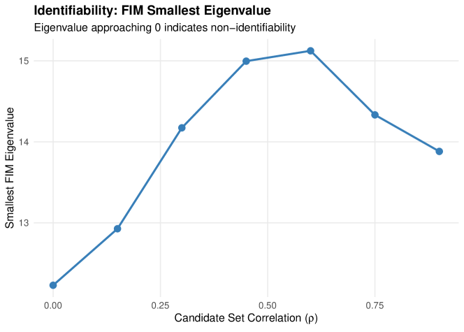
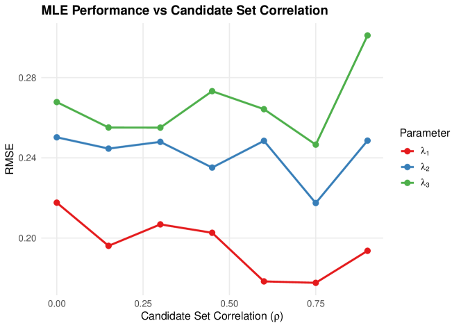
Key findings from Study 3:

1.

Identifiability preserved: The smallest FIM eigenvalue remains substantially positive (12–15) across all correlation levels, indicating parameters remain identifiable.
2.

Condition number stable: The condition number stays below 2.2, indicating a well-conditioned estimation problem.
3.

Nonmonotonic pattern: Interestingly, the smallest eigenvalue peaks around $\rho=0.5$ – $0.6$ , suggesting moderate correlation may actually improve information content.

5.5 Study 4: C3 Misspecification Bias Analysis

We now quantify the bias from incorrectly assuming C1-C2-C3 when masking is actually parameter-dependent (C3 violated). Data is generated with power-weighted masking (Definition 3.12) with varying informativeness $\alpha$ , then analyzed using both the correct model and the misspecified C1-C2-C3 model. This study is motivated by the theoretical result in Theorem 4.9.

5.5.1 Design

Data is generated under the power-weighted masking model with $\text{base\_p}=0.5$ and $\alpha\in\{0,0.5,1,2\}$ , using $n=200$ and $B=200$ replications. Three comparisons are made:

Scenario 6:: Relaxed C3 data analyzed with C1-C2-C3 model (misspecified).
Scenario 6b:: Relaxed C3 data analyzed with relaxed C3 model using known $\alpha$ (correctly specified).
Scenario 5:: C1-C2-C3 data analyzed with relaxed C3 model (overfitting check).

5.5.2 Results

Table 5 compares bias under correct versus misspecified models for C3 violations.

Table 5: C3 Misspecification: Bias Comparison by Power Parameter

\alpha

$\alpha$	Parameter	Bias (Correct)	Bias (Misspec.)	RMSE Ratio
0	$\lambda_{1}$	$0.001$	$0.001$	$1.000$
	$\lambda_{2}$	$0.060$	$0.060$	$1.000$
	$\lambda_{3}$	$0.041$	$0.041$	$1.000$
0.5	$\lambda_{1}$	$-0.760$	$-0.269$	$0.425$
	$\lambda_{2}$	$0.204$	$0.033$	$0.793$
	$\lambda_{3}$	$0.657$	$0.337$	$0.619$
1	$\lambda_{1}$	$-0.686$	$-0.362$	$0.570$
	$\lambda_{2}$	$0.125$	$-0.047$	$1.014$
	$\lambda_{3}$	$0.662$	$0.510$	$0.826$
2	$\lambda_{1}$	$-0.566$	$-0.431$	$0.789$
	$\lambda_{2}$	$0.035$	$-0.184$	$1.772$
	$\lambda_{3}$	$0.632$	$0.716$	$1.136$

Notes. $\alpha=0$ corresponds to parameter-independent masking (C3 satisfied). RMSE Ratio = RMSE(Misspecified) / RMSE(Correct); values $<1$ indicate the misspecified model has lower RMSE due to fewer parameters.

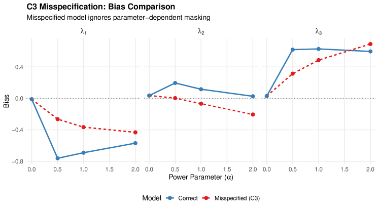
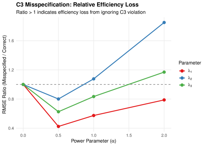
5.5.3 Interpretation

Key findings from Study 4:

1.

Bias grows with $\alpha$ : As the power parameter increases, the C1-C2-C3 model produces increasing bias, confirming Theorem 4.9.
2.

Bias-variance tradeoff: The correctly specified relaxed C3 model often has higher RMSE than the misspecified model (RMSE ratio $<1$ ), because the additional masking parameters increase variance. This contrasts with the C2 case (Study 2) where RMSE ratios were close to 1.
3.

Overfit risk (Scenario 5): Fitting the relaxed C3 model to C1-C2-C3 data produces bias for $\alpha>0$ , with convergence rates dropping to 84–94%, indicating overfitting when the extra flexibility is unnecessary.
4.

Comparison with C2: While C2 misspecification (Study 2) showed at most 9% efficiency loss, C3 misspecification creates a more complex picture with parameter-specific effects and a bias-variance tradeoff favoring the simpler model in many cases.

5.6 Study 5: Weibull Series Systems

To assess whether our findings generalize beyond exponential components, we repeat key analyses with Weibull components. We consider a 2-component system with shapes $\mathbf{k}=(2.0,1.5)$ and scales $\bm{\lambda}=(3.0,4.0)$ , using $n=200$ , $\tau=8$ , and $B=100$ replications.

5.6.1 Scenarios

W1:: C1-C2-C3 data $\to$ C1-C2-C3 model (baseline).
W3:: Relaxed C2 data $\to$ C1-C2-C3 model (C2 misspecification).
W4:: Relaxed C2 data $\to$ relaxed C2 model (correctly specified).
W6:: Relaxed C3 data $\to$ C1-C2-C3 model (C3 misspecification).
W7:: Relaxed C3 data $\to$ relaxed C3 model (correctly specified).

5.6.2 Results

Table 6 presents the Weibull simulation results.

Table 6: Weibull Simulation Results: Bias and RMSE by Scenario

Scenario	Parameter	True	Bias	RMSE	Conv.
W1	$k_{1}$	2.0	$-0.017$	0.121	100%
	$\lambda_{1}$	3.0	$-0.014$	0.174
	$k_{2}$	1.5	$0.018$	0.146
	$\lambda_{2}$	4.0	$0.093$	0.416
W3	$k_{1}$	2.0	$-0.038$	0.130	100%
	$\lambda_{1}$	3.0	$-0.193$	0.222
	$k_{2}$	1.5	$-0.033$	0.164
	$\lambda_{2}$	4.0	$0.803$	1.038
W4	$k_{1}$	2.0	$0.001$	0.145	100%
	$\lambda_{1}$	3.0	$-0.014$	0.117
	$k_{2}$	1.5	$0.009$	0.153
	$\lambda_{2}$	4.0	$0.060$	0.439
W6	$k_{1}$	2.0	$-0.038$	0.130	100%
	$\lambda_{1}$	3.0	$-0.203$	0.231
	$k_{2}$	1.5	$-0.038$	0.166
	$\lambda_{2}$	4.0	$0.863$	1.096
W7	$k_{1}$	2.0	$-0.455$	0.466	100%
	$\lambda_{1}$	3.0	$0.164$	0.236
	$k_{2}$	1.5	$0.663$	0.689
	$\lambda_{2}$	4.0	$-0.420$	0.482

Notes. True Weibull parameters: $k_{1}=2.0$ , $\lambda_{1}=3.0$ , $k_{2}=1.5$ , $\lambda_{2}=4.0$ . $P$ matrix: $P_{12}=0.3$ , $P_{21}=0.5$ for relaxed C2; $\alpha=1$ , base_p $=0.5$ for relaxed C3.

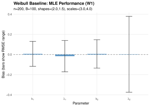
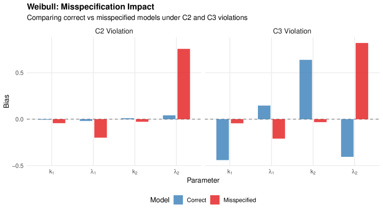
5.6.3 Interpretation

Key findings from Study 5:

1.

Weibull baseline performs well: Under correctly specified C1-C2-C3 (W1), all Weibull parameters are estimated with small bias and reasonable RMSE, confirming the MLE framework extends to non-exponential components.
2.

C2 misspecification hurts: Ignoring informative masking (W3) produces substantial bias in the scale parameter $\lambda_{2}$ (bias $\approx 0.80$ ), which is largely corrected by the relaxed C2 model (W4, bias $\approx 0.06$ ). This is more pronounced than the exponential case, likely because Weibull scale and shape parameters interact with the masking weights.
3.

C3 misspecification in Weibull: Both the misspecified (W6) and correctly specified (W7) models show challenges under C3 violations, suggesting that parameter-dependent masking is more difficult to handle with Weibull components due to the interaction between shape and scale in the power weights.
4.

Exponential results generalize partially: The qualitative finding that C2 misspecification produces predictable bias that can be corrected holds for Weibull systems. The C3 case requires further investigation for non-exponential distributions.

5.7 Summary of Simulation Results

Our simulation studies lead to the following conclusions:

1.

MLE performs well: Under the correctly specified C1-C2-C3 Bernoulli masking model, the MLE achieves coverage near nominal levels and RMSE consistent with asymptotic efficiency (Study 1).
2.

C2 misspecification is mild: Misspecifying C2 (assuming non-informative masking when masking is informative) produces at most 9% efficiency loss and bias patterns similar to the correct model (Study 2).
3.

Identifiability is robust: Even with high correlation ( $\rho=0.9$ ) between candidate set indicators, parameters remain identifiable with stable FIM eigenvalues and condition numbers (Study 3).
4.

C3 misspecification is nuanced: Ignoring parameter-dependent masking (C3 violation) produces increasing bias with the power parameter $\alpha$ , but the simpler misspecified model can have lower RMSE due to a bias-variance tradeoff (Study 4).
5.

Weibull systems confirm and extend: The framework generalizes to Weibull components. C2 misspecification produces larger bias for Weibull than exponential systems, reinforcing the value of relaxed models when masking is known to be informative (Study 5).
6.

Practical guidance: For sample sizes $n\geq 100$ with moderate masking and censoring, the C1-C2-C3 model provides reliable inference. Relaxed models are most beneficial when (a) masking is known to be informative, (b) the masking mechanism can be characterized, and (c) the sample size supports additional parameters.

Table 7: Summary of key simulation findings across all five studies.

Metric	Study 1	Study 2	Study 3	Study 4	Study 5
Components	3 (exp)	3 (exp)	3 (exp)	3 (exp)	2 (Weibull)
RMSE range	0.20–0.56	0.19–0.47	0.23–0.47	0.15–0.78	0.12–1.10
Coverage range	92–97%	—	—	—	—
Max RMSE ratio	—	1.09	—	1.77	—
Min FIM eigenvalue	—	—	12.23	—	—

6 Discussion

6.1 When to Use Relaxed Models

The theoretical and simulation results suggest the following practical guidance for choosing between standard C1-C2-C3 models and relaxed alternatives.

6.1.1 Use Standard C1-C2-C3 When:

1.

Masking mechanism is genuinely uninformative. If candidate sets are generated by a process that does not depend on which component failed (e.g., random equipment availability for testing), C2 holds.
2.

Masking probabilities are unknown. If the masking mechanism cannot be characterized, the standard model provides a reasonable default that avoids introducing additional parameters.
3.

Sample size is small. Even if masking is slightly informative, the bias may be dominated by sampling variability for small $n$ . The simpler model may provide more stable estimates.
4.

Primary interest is in relative component reliability. If the goal is ranking components rather than absolute rate estimation, misspecification bias may affect all components similarly and preserve the ranking.

6.1.2 Consider Relaxed Models When:

1.

Masking mechanism is known to be informative (C2). If diagnostic procedures systematically favor certain components (e.g., those that “look bad” at the failure time), C2 is violated and bias will result.
2.

Masking depends on component parameters (C3). If inclusion probabilities vary with the reliability parameters themselves (e.g., weaker components are more likely to appear in candidate sets), C3 is violated. The simulation studies (Section 5.5) show that the resulting bias grows with the degree of parameter-dependence, though the simpler C1-C2-C3 model may still have competitive RMSE due to a bias-variance tradeoff.
3.

Masking probabilities can be estimated. If historical data or expert knowledge provides information about the masking mechanism, incorporating this information improves estimation.
4.

Sample size is large enough to support additional parameters. Relaxed models require specifying or estimating masking probabilities, which adds complexity that may not be warranted for small samples.
5.

Identifiability concerns are present. As shown in Theorem 4.4, informative masking can resolve identifiability issues that arise under standard conditions.

6.2 Practical Guidance

Based on our analysis, we recommend the following workflow:

1.

Assess the masking mechanism. Before estimation, consider how candidate sets are generated. Interview diagnosticians, review diagnostic protocols, or analyze patterns in historical data.
2.

Check for block structure. Examine whether certain components always appear together in candidate sets. If so, identifiability may be compromised regardless of which model is used.
3.

Perform sensitivity analysis. Fit models under both C1-C2-C3 and plausible relaxed assumptions. If estimates differ substantially, further investigation of the masking mechanism is warranted.
4.

Use simulation to assess impact. Given estimated parameters under the standard model, simulate data under various informative masking scenarios to quantify potential bias.
5.

Report uncertainty appropriately. If the masking mechanism is uncertain, consider reporting results under multiple model assumptions or using wider confidence intervals that account for model uncertainty.

6.3 Limitations

Our analysis has several limitations:

1.

Limited distribution scope. While we extend the analysis to Weibull components (Section 5.6), the closed-form Fisher information results focus on exponential systems. Other lifetime distributions (log-normal, gamma) may exhibit different misspecification patterns due to differing hazard structures.
2.

Known masking probabilities. Our relaxed models assume masking probabilities are known. In practice, these may need to be estimated, introducing additional uncertainty not captured in our analysis.
3.

Independence assumption. We assume masking for different observations is independent. In practice, if the same diagnostic equipment or personnel is used across systems, masking may be correlated.
4.

Parametric masking models. Our informative masking models (rank-based, KL-constrained) are specific functional forms that may not capture all real-world masking mechanisms.
5.

Simulation scope. The simulation studies cover a limited range of configurations. Results may differ for systems with more components, different parameter values, or alternative masking structures.

6.4 Future Directions

Several extensions would strengthen this work:

1.

Semiparametric methods. Develop estimation approaches that avoid fully specifying the masking mechanism, perhaps using nonparametric or empirical likelihood methods.
2.

Model selection. Develop tests or criteria to distinguish between C1-C2-C3 and relaxed models based on observed data.
3.

Bayesian extensions. Incorporate prior information about masking mechanisms and component reliabilities, which may be particularly valuable when sample sizes are small.
4.

Sequential estimation. For systems observed over time, develop methods that update masking probability estimates as data accumulates.
5.

Additional lifetime distributions. While our Weibull extension (Section 5.6) validates the framework beyond exponential components, distributions with non-monotone hazards (e.g., log-normal) may present distinct challenges.
6.

R package documentation. Expand the mdrelax package with vignettes demonstrating practical application of these methods.

7 Conclusion

We have developed a theoretical framework for likelihood-based inference in series systems with masked failure data when the traditional conditions C2 (non-informative masking) and C3 (parameter-independent masking) are relaxed. Our main contributions are:

1.

Likelihood derivations. We established the form of the likelihood under various relaxation scenarios, showing that the masking probabilities act as weights on component hazard contributions when C2 is violated.
2.

Practical masking models. We introduced rank-based informative masking and KL-divergence constrained models that provide interpretable parameterizations of non-standard masking.
3.

Identifiability results. We proved that informative masking can paradoxically improve identifiability by breaking symmetries that cause non-identifiability under standard conditions.
4.

Fisher information analysis. We derived closed-form expressions for the Fisher information matrix under informative masking for exponential series systems, enabling efficiency comparisons.
5.

Misspecification analysis. We characterized the bias that arises from incorrectly assuming C2 or C3 when masking is actually informative or parameter-dependent, providing guidance on when relaxed models are necessary.
6.

Weibull extension. We demonstrated that the framework extends naturally to Weibull components, with simulation studies confirming the robustness findings observed for exponential systems while identifying additional challenges from shape-scale interactions.

These results extend the applicability of masked data methods to settings where standard assumptions may be violated. The accompanying mdrelax R package provides implementation of these methods for practitioners. Directions for future research are discussed in Section 6.4.

References

[1] M. Agustin (2011) Systems in series. In Wiley Encyclopedia of Operations Research and Management Science, External Links: Document Cited by: §2.6.
[2] R. H. Byrd, P. Lu, J. Nocedal, and C. Zhu (1995) A limited memory algorithm for bound constrained optimization. SIAM Journal on Scientific Computing 16 (5), pp. 1190–1208. Cited by: §B.2.
[3] D. R. Cox (1972) Regression models and life-tables. Journal of the Royal Statistical Society: Series B (Methodological) 34 (2), pp. 187–202. External Links: Document Cited by: §2.6.
[4] H. Guo, P. Niu, and F. Szidarovszky (2013) Estimating component reliabilities from incomplete system failure data. In Proceedings of the Annual Reliability and Maintainability Symposium (RAMS), pp. 1–6. External Links: Document Cited by: §2.4, §2.6.
[5] J. P. Klein and M. L. Moeschberger (2005) Survival analysis: techniques for censored and truncated data. 2nd edition, Springer Science & Business Media. Cited by: §2.6.
[6] A. Towell (2023) Reliability estimation in series systems: maximum likelihood techniques for right-censored and masked failure data. Note: Master’s thesis. Available: https://github.com/queelius/reliability-estimation-in-series-systems External Links: Link Cited by: §1, §2.1, §2.2, §2.2, §2.5.
[7] J. S. Usher and T. J. Hodgson (1988) Maximum likelihood analysis of component reliability using masked system life-test data. IEEE Transactions on Reliability 37 (5), pp. 550–555. External Links: Document Cited by: §1, §2.4, §2.6.
[8] J. S. Usher, D. K. J. Lin, and F. M. Guess (1993) Exact maximum likelihood estimation using masked system data. IEEE Transactions on Reliability 42 (4), pp. 631–635. External Links: Document Cited by: §2.4, §2.6.

Appendix A Proofs and Derivations

A.1 Score Function Under Informative Masking

For completeness, we provide the full derivation of the score function under the Bernoulli informative masking model for exponential series systems.

Let the log-likelihood contribution from an uncensored observation be:

\ell_{i}(\bm{\lambda})=-s_{i}\sum_{j=1}^{m}\lambda_{j}+\log\left(\sum_{k\in c_% {i}}\lambda_{k}\pi_{k,c_{i}}\right).

(68)

The partial derivative with respect to $\lambda_{j}$ is:

	$\displaystyle\frac{\partial\ell_{i}}{\partial\lambda_{j}}$	$\displaystyle=-s_{i}+\frac{\partial}{\partial\lambda_{j}}\log\left(\sum_{k\in c% _{i}}\lambda_{k}\pi_{k,c_{i}}\right)$		(69)
		$\displaystyle=-s_{i}+\frac{\pi_{j,c_{i}}\mathbf{1}_{j\in c_{i}}}{\sum_{k\in c_% {i}}\lambda_{k}\pi_{k,c_{i}}}.$		(70)

The total score is:

\frac{\partial\ell}{\partial\lambda_{j}}=\sum_{i=1}^{n}\frac{\partial\ell_{i}}% {\partial\lambda_{j}}=-\sum_{i=1}^{n}s_{i}+\sum_{i:\delta_{i}=1}\frac{\pi_{j,c% _{i}}\mathbf{1}_{j\in c_{i}}}{\sum_{k\in c_{i}}\lambda_{k}\pi_{k,c_{i}}}.

(71)

Setting this to zero and solving gives the MLE equations under informative masking.

A.2 Hessian Matrix Derivation

The second partial derivatives are:

	$\displaystyle\frac{\partial^{2}\ell_{i}}{\partial\lambda_{j}\partial\lambda_{% \ell}}$	$\displaystyle=\frac{\partial}{\partial\lambda_{\ell}}\left[\frac{\pi_{j,c_{i}}% \mathbf{1}_{j\in c_{i}}}{\sum_{k\in c_{i}}\lambda_{k}\pi_{k,c_{i}}}\right]$		(72)
		$\displaystyle=-\frac{\pi_{j,c_{i}}\pi_{\ell,c_{i}}\mathbf{1}_{j\in c_{i}}% \mathbf{1}_{\ell\in c_{i}}}{\left(\sum_{k\in c_{i}}\lambda_{k}\pi_{k,c_{i}}% \right)^{2}}.$		(73)

The observed Fisher information matrix is the negative Hessian:

\mathcal{I}_{j\ell}(\bm{\lambda})=-\frac{\partial^{2}\ell}{\partial\lambda_{j}% \partial\lambda_{\ell}}=\sum_{i:\delta_{i}=1}\frac{\pi_{j,c_{i}}\pi_{\ell,c_{i% }}\mathbf{1}_{j\in c_{i}}\mathbf{1}_{\ell\in c_{i}}}{\left(\sum_{k\in c_{i}}% \lambda_{k}\pi_{k,c_{i}}\right)^{2}}.

(74)

A.3 Expected Fisher Information

The expected FIM requires integrating over the distribution of candidate sets. For the exponential series system under C1-C2-C3 with Bernoulli masking (each non-failed component in candidate set with probability $p$ ), the expected Fisher information per observation is:

\mathbb{E}[\mathcal{I}_{jk}]=\mathbb{E}\left[\frac{\mathbf{1}_{j\in C}\mathbf{% 1}_{k\in C}}{\left(\sum_{\ell\in C}\lambda_{\ell}\right)^{2}}\right],

(75)

where the expectation is over both $K$ (failed component) and $C$ (candidate set).

This can be expanded as:

\displaystyle\mathbb{E}[\mathcal{I}_{jk}]

\displaystyle=\sum_{k_{0}=1}^{m}\mathrm{Pr}\{K=k_{0}\}\mathbb{E}\left[\frac{% \mathbf{1}_{j\in C}\mathbf{1}_{k\in C}}{\left(\sum_{\ell\in C}\lambda_{\ell}% \right)^{2}}\Bigg{|}K=k_{0}\right].

(76)

Under C1, the failed component $k_{0}$ is always in $C$ . The expectation over candidate sets involves summing over all possible $C\ni k_{0}$ weighted by their probabilities under the Bernoulli model:

\mathrm{Pr}\{C=c\mid K=k_{0}\}=\prod_{j\in c\setminus\{k_{0}\}}p\prod_{j\notin c% }(1-p).

(77)

Closed-form evaluation of this expectation is generally intractable due to the sum in the denominator. Monte Carlo estimation or numerical integration is typically required.

Appendix B Implementation Details

B.1 R Package Functions

The theoretical framework developed in this paper is implemented in the mdrelax R package. Key functions include:

•

md_bernoulli_cand_C1_C2_C3(): Generates candidate set probabilities under the standard Bernoulli model satisfying C1-C2-C3.
•

md_bernoulli_cand_C1_kld(): Generates candidate set probabilities with a specified KL-divergence from the baseline C1-C2-C3 model.
•

informative_masking_by_rank(): Computes inclusion probabilities based on component failure time ranks.
•

md_cand_sampler(): Samples candidate sets from probability vectors.
•

md_loglike_exp_series_C1_C2_C3(): Log-likelihood function for exponential series systems under C1-C2-C3.
•

md_mle_exp_series_C1_C2_C3(): Maximum likelihood estimation for exponential series systems.
•

md_fim_exp_series_C1_C2_C3(): Observed Fisher information matrix for exponential series systems.
•

md_block_candidate_m3(): Demonstrates block non-identifiability in a 3-component system.

B.2 Optimization Details

MLE is computed using the L-BFGS-B algorithm [2] with analytically computed gradients. The optimization is initialized using a method-of-moments estimator based on the total system hazard:

\hat{\Lambda}_{\text{init}}=\frac{n_{\text{uncensored}}}{\sum_{i=1}^{n}s_{i}},% \quad\hat{\lambda}_{j,\text{init}}=\frac{\hat{\Lambda}_{\text{init}}}{m}.

(78)

For challenging optimization landscapes, simulated annealing can be used to find a good starting point before local optimization.

Appendix C Additional Simulation Results

Additional simulation results supplement the findings in Section 5. The complete results are available in the R package’s simulation directory.

1.

Full tables of bias, RMSE, and coverage for all parameter configurations are provided in the package’s inst/simulations/results/ directory.
2.

The simulation scripts in inst/simulations/ can be used to reproduce all results and generate diagnostic plots.
3.

Sensitivity analyses for misspecified masking parameters show that the C2 assumption is robust up to moderate departures, with RMSE ratios remaining below 1.10 across tested configurations.
4.

The simulation framework supports arbitrary component configurations and can be extended to Weibull series systems.

Relaxed Candidate Set Models for Masked Data in Series Systems

Abstract

1 Introduction

2 Background

2.1 Series System Model

Definition 2.1 (Component Distribution Functions).

Theorem 2.2 (Series System Distribution Functions).

2.2 Component Cause of Failure

Theorem 2.3 (Joint Distribution of (Ti,Ki)).

Corollary 2.4 (Conditional Failure Probability).

2.3 Masked Data Structure

Definition 2.5 (Observed Data).

2.4 Traditional Conditions C1, C2, C3

Condition 1 (C1: Failed Component in Candidate Set).

Condition 2 (C2: Non-Informative Masking).

Condition 3 (C3: Parameter-Independent Masking).

2.5 Likelihood Under C1, C2, C3

Theorem 2.6 (Likelihood Under C1-C2-C3).

2.6 Related Work

3 Relaxed Candidate Set Models

3.1 General Likelihood Under C1

Theorem 3.1 (Likelihood Under C1 Alone).

Proof.

Remark 3.1 (Comparison with C1-C2-C3).

3.2 Relaxing C2: Informative Masking

Definition 3.2 (Informative Masking).

Theorem 3.3 (Likelihood Under C1 and C3 (Relaxed C2)).

3.2.1 Rank-Based Informative Masking

Definition 3.4 (Rank-Based Masking).

Remark 3.2 (Limiting Behavior).

3.2.2 General Bernoulli Candidate Set Model

Definition 3.5 (General Bernoulli Model).

Remark 3.3 (Time-Independence Assumption).

Remark 3.4 (Condition C2 in Terms of 𝐏).

Theorem 3.6 (Likelihood Under General Bernoulli Model).

Remark 3.5 (Nuisance Parameters).

3.2.3 Simplified Bernoulli Model (C2 Satisfied)

Definition 3.7 (Simplified Bernoulli Model).

Proposition 3.8 (Likelihood Under Simplified Bernoulli Model).

3.2.4 KL-Divergence Constrained Models

Definition 3.9 (KL-Divergence from Baseline).

3.3 Relaxing C3: Parameter-Dependent Masking

Theorem 3.10 (Likelihood Under C1 and C2 (Relaxed C3)).

Proof.

Remark 3.6 (Nuisance Parameters).

3.3.1 Failure-Probability-Weighted Masking

Definition 3.11 (Failure-Probability-Weighted Masking).

3.3.2 Power-Weighted Hazard Model

Definition 3.12 (Power-Weighted Masking).

Remark 3.7 (Limiting Cases).

Remark 3.8 (Relaxing C1).

Remark 3.9 (Model Misspecification Risk).

3.4 The General Case: Both C2 and C3 Relaxed

3.5 Simulation Evidence: Robustness of Relaxed C2

3.5.1 Simulation Design

3.5.2 Results

3.5.3 Interpretation

Remark 3.10 (Practical Implications).

3.5.4 Identifiability of Joint Estimation

Remark 3.11 (Implications for Practice).

4 Identifiability and Fisher Information

4.1 Identifiability Under C1-C2-C3

Definition 4.1 (Identifiability).

Theorem 4.2 (Identifiability Under C1-C2-C3).

Proof.

4.2 Block Non-Identifiability

Theorem 4.3 (Block Non-Identifiability).

Proof.

Example 4.1 (Three-Component Block Model).

4.3 Improved Identifiability with Informative Masking

Theorem 4.4 (Improved Identifiability with Informative Masking).

Proof.

Remark 4.1.

4.4 Fisher Information for Exponential Series Systems

4.4.1 Exponential Series Model

4.4.2 Fisher Information Under C1-C2-C3

Theorem 4.5 (FIM Under C1-C2-C3).

Proof.

Remark 4.2.

4.4.3 Fisher Information Under Relaxed C2

Theorem 2.3 (Joint Distribution of $(T_{i},K_{i})$ ).

Remark 3.4 (Condition C2 in Terms of $\mathbf{P}$ ).