Time Series Analysis of Confidentiality Degradation in Encrypted Search Systems
Abstract
We present a tutorial-style analysis of confidentiality degradation in encrypted search systems subject to known-plaintext attacks. We first develop an intuitive explanation of why frequency-based attacks succeed, connecting the entropy of the plaintext distribution to the rate of adversary learning. A worked example with a small vocabulary illustrates the attack mechanism step-by-step. We then model the adversary’s accuracy as a time-dependent confidentiality measure and develop forecasting models based on ARIMA and dynamic regression techniques. Our analysis provides quantitative estimates for how quickly adversary knowledge accumulates, enabling organizations to establish data-driven policies for password rotation and system reinitialization that maintain specified confidentiality thresholds. We conclude with key insights for practitioners, including the fundamental role of query entropy and guidelines for interpreting wide prediction intervals.
1 Introduction
Cloud computing enables organizations to store and process data on remote infrastructure, but this convenience comes at the cost of reduced control over data confidentiality. Even when data is encrypted at rest, system administrators and other insiders pose a significant threat. This tension between utility and security has motivated the development of encrypted search systems.
Encrypted search attempts to resolve the fundamental trade-off between confidentiality and usability by enabling authorized users to query encrypted data without revealing query contents to untrusted parties.
Definition 1.
Encrypted search allows authorized search agents to investigate the presence of specific search terms in a confidential target data set, such as a database of encrypted documents, while the contents—especially the meaning of the target data set and search terms—are hidden from unauthorized personnel, including the system administrators of a cloud server.
Essentially, encrypted search enables oblivious queries where users can search confidential databases on untrusted systems without revealing their information needs (and in more sophisticated systems, without revealing which documents matched the query).
We define the adversary as any untrusted party with access to the remote system where confidential data is stored.111System administrators are typical examples.
However, perfect confidentiality is not achievable in practice. Encrypted search systems leak information through access patterns, query frequencies, and other side channels. In this paper, we focus on an adversary who attempts to infer the plaintext queries by analyzing the history of encrypted searches using a known-plaintext attack.
We quantify confidentiality using the proportion of queries the adversary successfully decodes. Since confidentiality degrades as the adversary observes more queries, we model this degradation as a time series process.
Time series analysis enables us to forecast future confidentiality levels, answering critical security questions such as: How long until confidentiality falls below an acceptable threshold? When should passwords be reset to maintain a minimum confidentiality level?
These forecasts support data-driven security policies. Password resets impose usability and security costs, but delaying them risks unacceptable confidentiality loss. Our analysis provides quantitative guidance for balancing these competing concerns.
2 Related work
Searchable encryption was introduced by Song, Wagner, and Perrig [6], who developed practical techniques for searching on encrypted data while preserving query confidentiality. Their foundational work demonstrated that encrypted search systems could achieve practical performance, but acknowledged that such systems necessarily leak some information through access patterns and query frequencies.
Subsequent research has shown that these information leakages enable significant attacks. Islam et al. [4] demonstrated access pattern disclosure attacks that exploit the deterministic nature of encrypted search schemes. By observing which encrypted documents match encrypted queries, an adversary can infer plaintext queries even without directly observing query contents. Their attack model closely parallels our known-plaintext attack framework: both exploit frequency analysis and co-occurrence patterns in the query stream to recover plaintext information. While Islam et al. focused on one-time attacks, our work extends this perspective by modeling confidentiality degradation as a time series process, enabling forecasts of when adversary knowledge will violate security thresholds.
3 Encrypted search model
In information retrieval, a search agent submits a query representing an information need to an information system, which responds with relevant objects (e.g., documents).
We make the following simplifying assumptions about the query model and encryption scheme.
Assumption 1.
Queries consist of sequences of keywords (a bag-of-words model).
Assumption 2.
The encrypted search system uses a deterministic encryption scheme where each plaintext keyword maps to a unique encrypted token (trapdoor).
More formally, we define the encryption function as
| (1) |
where is the set of plaintext search keywords and is the set of encrypted tokens (trapdoors).
Definition 2 (Trapdoor).
A trapdoor is a cryptographic token generated by applying to a plaintext keyword, enabling the untrusted system to perform searches without learning the plaintext.
Since is injective, there exists an inverse function
| (2) |
such that for every .
Definition 3.
The adversary can observe the sequence of encrypted queries (trapdoors) submitted by authorized search agents but does not initially know .
The security objective is to prevent the adversary from learning and thus decoding the queries.
We now formalize the time series notation. Following standard conventions, we use uppercase letters for random variables and lowercase for realizations. A time series denotes a sequence of random variables indexed by time , with denoting an observed realization.
The plaintext queries form a discrete-time, discrete-valued time series where is the -th keyword submitted by search agents. The adversary cannot observe directly.
Definition 4.
The encrypted query sequence is defined by
where is the trapdoor corresponding to plaintext .
We model queries probabilistically as a random process with distribution determined by a language model:
| (3) |
This formulation assumes queries depend only on query history, not on external factors such as user identity or time of day. We discuss extensions to include such covariates in Section 8.
The encrypted query sequence is then modeled as the random process where .
4 Threat model: known-plaintext attack
The adversary observes the encrypted query sequence and attempts to recover the plaintext sequence by learning the decryption function . We focus on frequency-based cryptanalysis, specifically known-plaintext attacks. Side-channel information is not considered in this work; we discuss potential extensions in Section 8.
Assumption 3.
The decryption function is unknown to the adversary.
The adversary’s strategy is to estimate by exploiting statistical properties of natural language. Given observed ciphers , a maximum likelihood estimator of is
| (4) |
where denotes the set of all injective functions from to .
Perfect confidentiality would require that all plaintexts be equally likely, making them indistinguishable to the adversary. In this case, would be inconsistent. However, natural language exhibits strong statistical regularities (word frequencies follow Zipf’s law, co-occurrence patterns are non-uniform), enabling the adversary to learn something about from .
In practice, the adversary does not know the true distribution of but can approximate it using external corpora.
Assumption 4.
The adversary has access to an approximate language model for the query distribution.
Definition 5.
In a known-plaintext attack, the adversary estimates by solving the MLE in Equation (4) with the true distribution replaced by the approximate distribution .
The quality of the attack depends on how well approximates the true query distribution.
4.1 Why frequency matching works
The success of frequency-based attacks rests on a fundamental insight: the adversary’s task becomes easier when the plaintext distribution has low entropy. We now explain why this is the case.
Consider the simplified attack strategy of frequency matching: the adversary ranks observed ciphers by their frequency counts and matches them to the corresponding ranks in the known plaintext distribution. For example, if cipher appears most frequently, the adversary guesses it corresponds to the most common plaintext word.
This strategy succeeds when empirical frequencies preserve the true ranking. By the law of large numbers, observed frequencies converge to true probabilities as more queries are observed. The key question is: how quickly?
Conjecture 1 (Convergence of Frequency Matching).
Let be a discrete distribution over words with probabilities . After observing samples, the probability that word is correctly ranked (i.e., has empirical frequency rank equal to its true rank) increases with and with the gap .
A formal proof with explicit convergence rates is left for future work; the intuition is developed below.
The intuition is straightforward: if word has probability 0.1 and word has probability 0.01, then after observations we expect approximately occurrences of and occurrences of . For large , will almost certainly have a higher count than . The frequency matching attack succeeds when such orderings are preserved for all word pairs.
4.1.0.1 The role of entropy.
Low-entropy distributions have probability mass concentrated in a few high-frequency words. This concentration creates large gaps between adjacent word probabilities, enabling faster convergence of the frequency matching attack.
Let denote the Shannon entropy of the plaintext distribution [1]. The adversary’s information gain after observing queries, relative to a uniform prior, is quantified by:
| (5) |
When is small (concentrated distribution), each observation provides substantial information. When (uniform distribution), observations provide minimal information about word identities.
This quantity represents the mutual information between the observed cipher sequence and the plaintext identities, accumulated over observations. When queries are i.i.d., the per-query information gain is exactly bits [1].
Remark (Information-Theoretic Interpretation).
Equation (5) reveals a fundamental security parameter: the entropy gap determines the rate of confidentiality degradation. Systems with high-entropy query distributions (diverse, unpredictable queries) degrade slowly; systems with low-entropy distributions (repetitive, predictable queries) degrade rapidly.
4.1.0.2 Zipf’s law and natural language.
Natural language word frequencies follow Zipf’s law [7]: the probability of the -th most common word is proportional to for some exponent . For English text, . Table 1 illustrates how the Zipf exponent affects entropy and attack speed.
| Zipf | Entropy (bits) | Attack Speed | Interpretation |
|---|---|---|---|
| 0 | 13.3 (maximum) | Slowest | Uniform queries |
| 0.5 | Medium | Moderate skew | |
| 1.0 | Faster | Typical Zipfian text | |
| Very fast | Highly predictable |
This analysis yields a key design principle: encrypted search systems should encourage query diversity (high entropy) to slow adversary learning.
5 Confidentiality measure
We quantify confidentiality degradation using the adversary’s decryption accuracy.
Definition 6.
The confidentiality measure is defined as the fraction of ciphers correctly decoded by the adversary using :
| (6) |
where
| (7) |
Here is a sampling parameter: we compute one measurement of after every queries.
The measure represents the proportion of the entire query history that the adversary can decode at time . Note that increases as the adversary observes more queries and refines .
5.1 Illustrative example
To build intuition, we trace through one step of the frequency matching attack on a small vocabulary.
5.1.0.1 Setup.
Consider a vocabulary of words with a Zipf-like probability distribution:
| Word | apple | banana | cherry | date | elderberry |
|---|---|---|---|---|---|
| Probability | 0.40 | 0.25 | 0.20 | 0.10 | 0.05 |
| True rank | 1 | 2 | 3 | 4 | 5 |
The entropy is bits, well below the maximum bits for a uniform distribution.
5.1.0.2 Encryption.
The encryption function maps each word to a cipher, but the adversary does not know this mapping:
5.1.0.3 Adversary observation.
After observing 100 encrypted queries, the adversary counts cipher frequencies:
| Cipher | |||||
|---|---|---|---|---|---|
| Count | 42 | 23 | 19 | 11 | 5 |
| Observed rank | 1 | 2 | 3 | 4 | 5 |
5.1.0.4 Frequency matching attack.
The adversary matches observed ranks to known word ranks:
In this example, the adversary correctly identifies all five words because the observed frequency ordering matches the true probability ordering.
5.1.0.5 Confidentiality measure.
Since all words are correctly decoded:
The adversary has achieved complete recovery.
5.1.0.6 Key insight.
The attack succeeded quickly (only 100 queries) because the distribution has low entropy—high-probability words like “apple” dominate early observations, making frequency matching reliable. With a more uniform distribution, the attack would require many more observations to distinguish word frequencies.
5.1.0.7 When frequency matching fails.
In practice, words with similar probabilities may swap rankings due to sampling variance. For instance, if “banana” (0.25) and “cherry” (0.20) had counts of 21 and 22 respectively, the adversary would incorrectly swap their identities. The confidentiality measure would then be (only three words correct). Such partial failures are common when probability gaps are small.
5.2 Security threshold and password rotation
Suppose we require that confidentiality remain above a threshold . We define the critical time as
| (8) |
At time , the adversary can decode more than proportion of queries, violating the security requirement.
To maintain the threshold, we must reinitialize the encryption before reaching . This typically involves changing the cryptographic key (e.g., requiring password changes), which generates a new encryption function and resets the adversary’s knowledge. The adversary must then restart the attack process with .
Forecasting enables proactive security policies: we can predict when will exceed and schedule reinitialization accordingly.
5.3 Forecasting model
Since is random, the confidentiality measure is also random. We model it as a stochastic process .
Given observations , the -step ahead forecast distribution is
The forecast mean is denoted .
Our goal is to estimate the forecast distribution from observed data. In practice, we estimate the forecast mean and construct prediction intervals using the estimated forecast variance.
6 Data description
We analyze simulated data to evaluate forecasting models for . The simulation generates realistic query sequences and models an adversary conducting a known-plaintext attack.
6.1 Data generation
The simulation proceeds in two phases: query generation and attack simulation.
6.1.0.1 Query generation.
We first generate a synthetic plaintext query sequence :
-
1.
A bigram language model is estimated from a text corpus. (The original corpus is being recovered; it was a general English text collection. This limitation notwithstanding, the methodology demonstrated here applies to any corpus following Zipfian statistics.)
-
2.
Plaintext queries are sampled from this bigram model.
-
3.
Each plaintext is encrypted via a cryptographic hash function to produce ciphers .
6.1.0.2 Attack simulation.
Given the cipher sequence , we simulate an adversary attempting to learn :
-
1.
After every ciphers, the adversary updates its estimate by solving a unigram MLE:
Note that the adversary uses a unigram model even though queries were generated from a bigram model. This reflects information loss in practice.
-
2.
The adversary’s language model is estimated from a different corpus than the one used to generate . This mismatch makes inconsistent (it does not converge to as ), reflecting realistic conditions where the adversary’s knowledge is imperfect.
-
3.
The confidentiality measure is computed using the current estimate .
This setup models a realistic scenario where the adversary has approximate but not perfect knowledge of the query distribution.
7 Time series analysis of
The adversary’s accuracy exhibits temporal dependence: accuracy at time is correlated with recent values , with correlation typically decreasing as lag increases. This autocorrelation structure motivates time series methods for forecasting.
We partition the data into training and test sets. The training set is used for model fitting and the test set is held out for evaluation. Sample training data:
## [1] 0.358159 0.351208 0.347271 0.346403 0.352666 0.350445
7.1 Visualization and stationary transformations
ARIMA models assume stationarity: constant mean, constant variance, and autocorrelation that depends only on lag. We must transform to approximate stationarity before fitting ARIMA models.
Figure 1 plots the training data. The series exhibits an upward trend, indicating non-stationarity in the mean.

Figure 2 shows the sample ACF and PACF. The slow decay in the ACF confirms non-stationarity.
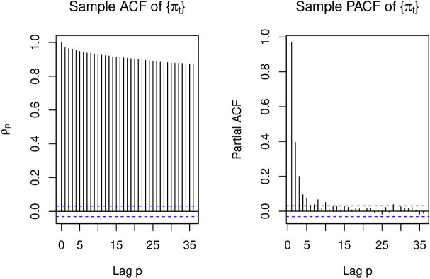
The variance appears reasonably constant, so variance-stabilizing transformations (e.g., logarithm) are unnecessary. To remove the trend, we apply differencing: the -th order differenced series is denoted . Differencing is a flexible, non-parametric approach that adapts to complex trend patterns without assuming a specific functional form.

Figure 3 shows the differenced series . The trend is removed, values fluctuate around zero, and variance appears constant. This suggests stationarity.
We apply the augmented Dickey-Fuller test [2] to formally test for stationarity:
## Augmented Dickey-Fuller Test
## Dickey-Fuller = -20.37, Lag order = 15, p-value = 0.01
## alternative hypothesis: stationary
The -value of 0.01 provides strong evidence against the null hypothesis of non-stationarity. We conclude that is approximately stationary and proceed with ARIMA modeling.
7.2 ARIMA model selection
Our goal is to build a parsimonious forecasting model. Following Occam’s razor, simpler models with fewer parameters are preferred: they generalize better to unseen data and avoid overfitting [3]. However, the model must be sufficiently complex to capture the data’s structure. This is the classical bias-variance tradeoff [3].
ARIMA models are parameterized by three integers: (autoregressive order), (differencing order), and (moving average order). We seek small values of , , and that adequately fit the data. While information criteria like AIC can guide selection, we also examine diagnostic plots.
Figure 4 shows the ACF and PACF of .
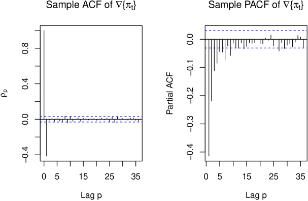
The ACF cuts off after lag 1, and the PACF decays exponentially, suggesting an MA(1) process for (i.e., IMA(1,1) for ).
The extended ACF (EACF) table provides additional guidance:
## AR/MA
##   0 1 2 3 4 5 6 7 8 9 10 11 12 13
## 0 x o o o o o o x x x o  o  o  o
## 1 x x o o o o x o o o o  o  o  o
## 2 x x x o o o x o o o o  o  o  o
## 3 x x x x o o o o o o o  o  o  o
## 4 x x x x x o o o o o o  o  o  o
## 5 x x x x x x o o o o o  o  o  o
## 6 x x x x x o x o o o o  o  o  o
## 7 x x x x x x x o o o o  o  o  o
The EACF suggests candidate models ARMA, ARMA, and ARMA for . We evaluate all three.
7.3 Model construction and evaluation
Model adequacy is assessed through residual diagnostics. A well-specified model produces residuals that behave like white noise:
-
1.
Uncorrelated: If residuals are correlated, the model has not captured all temporal structure and can be improved.
-
2.
Zero mean: Non-zero mean residuals indicate systematic bias in forecasts.
-
3.
Constant variance: Heteroscedasticity may require variance modeling.
7.3.1 IMA(1,1)
We first fit ARIMA, the simplest candidate model. The estimated parameter is:
##        ma1
## -0.5705635
Figure 5 shows residual diagnostics.
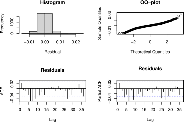
The histogram appears symmetric around zero, but the Q-Q plot shows deviations from normality. More critically, the ACF and PACF exhibit significant residual autocorrelation, indicating the model has not captured all temporal dependence. We reject this model.
7.3.2 IMA(1,2)
Next we fit ARIMA. The estimated parameters are:
##         ma1         ma2
## -0.55254743 -0.04124893
Figure 6 shows residual diagnostics.
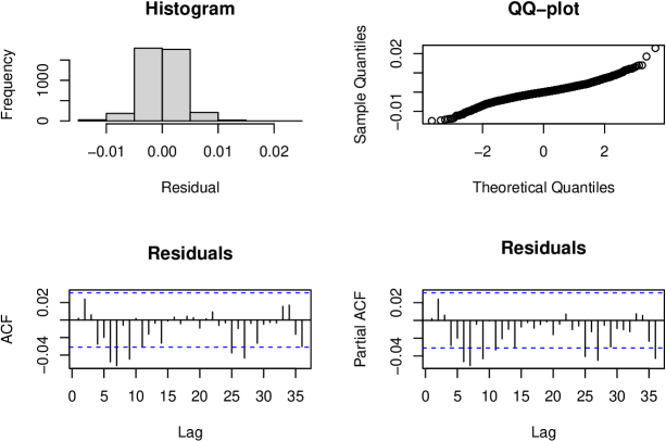
As before, the histogram is symmetric, and the Q-Q plot indicates non-normality (though normality is not strictly required for forecasting). However, the ACF and PACF again show significant residual correlation. This model is also inadequate. We reject it.
7.3.3 ARIMA(1,1,2)
Finally, we fit ARIMA. The estimated parameters are:
##        ar1        ma1        ma2
##  0.8839643 -1.4423574  0.4689439
Figure 7 shows residual diagnostics.
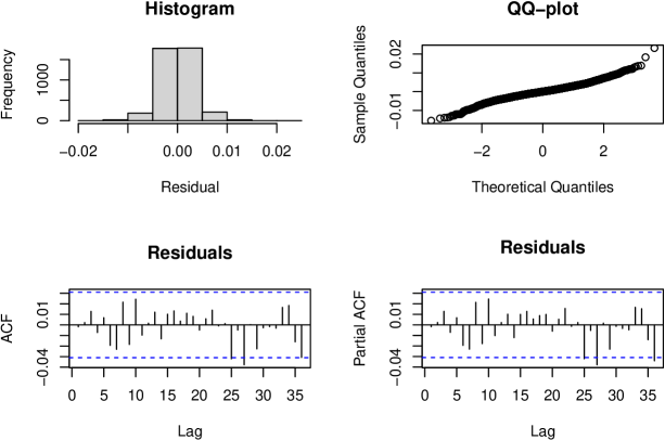
Again, the histogram is symmetric and the Q-Q plot shows non-normality. However, the ACF and PACF appear acceptable: no significant residual autocorrelation is evident.
We apply the Ljung-Box test (lag 10) to formally assess the white noise hypothesis:
## Box-Ljung test
## data: model.3$residuals
## X-squared = 10.333, df = 7, p-value = 0.1705
The null hypothesis is that residuals are white noise. The -value of 0.171 provides substantial support for this hypothesis.
We select ARIMA as our model. Since this is the only model passing diagnostics, formal comparison via AIC is unnecessary.
The fitted model summary is:
## ARIMA(1,1,2)
##
## Coefficients:
##          ar1      ma1     ma2
##       0.8840  -1.4424  0.4689
## s.e.  0.0276   0.0338  0.0266
##
## sigma^2 estimated as 1.088e-05:  log likelihood=17177.64
## AIC=-34347.27   AICc=-34347.26   BIC=-34322.1
In operator form, the model is
| (9) |
which factors as
| (10) |
where with .
7.4 Forecasting
We now use the fitted ARIMA model to forecast future confidentiality degradation. At time , we compute forecasts for .
Figure 8 shows the forecast along with 80% prediction intervals.
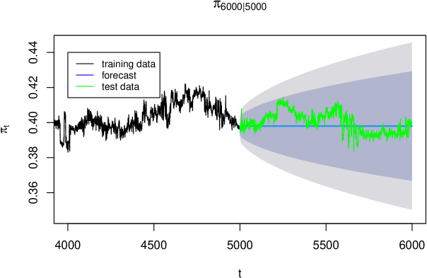
The held-out test data falls within the 80% prediction interval for most time points, suggesting reasonable forecast performance. However, the prediction intervals are quite wide. We hypothesize this reflects model misspecification: the purely autoregressive structure may not capture the underlying process adequately. Theoretically, should approach an asymptotic limit as the adversary’s knowledge saturates, but the ARIMA model does not incorporate this constraint. We explore theory-driven models in the next section.
7.5 Incorporating a priori information
We now incorporate domain knowledge about the confidentiality measure. Assuming the plaintext distribution and encryption function remain fixed, we expect:
-
1.
(it is a proportion).
-
2.
should be monotonically increasing: observing more queries cannot decrease the adversary’s accumulated knowledge.
-
3.
should approach an asymptotic limit as the adversary’s knowledge saturates.
These properties suggest models like Gompertz growth curves or scaled CDFs. For simplicity, we approximate the trend with a logarithmic function:
| (11) |
While this lacks an asymptote, it provides a reasonable approximation over finite time horizons.
We model deviations from this trend as ARIMA errors:
| (12) |
where .
Note that this formulation (regression with ARIMA errors) differs from standard regression. As Hyndman [5] notes, the regression coefficients condition on lagged responses, complicating interpretation. Nevertheless, this model can improve forecasts by capturing both the deterministic trend and stochastic dynamics.
We fit this model to the data:
## Regression with ARIMA(1,1,2) errors
##
## Coefficients:
##          ar1      ma1     ma2    xreg
##       0.8521  -1.4012  0.4355  0.0292
## s.e.  0.0234   0.0277  0.0211  0.0202
##
## sigma^2 estimated as 6.828e-06:  log likelihood=45279.87
## AIC=-90549.73   AICc=-90549.73   BIC=-90513.68
This uses ARIMA errors with a logarithmic trend term. (We also tested ARIMA, which yielded tighter prediction intervals but was not substantially better.)
Figure 9 shows residual diagnostics.
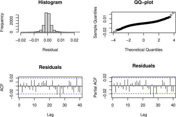
The histogram is symmetric, the Q-Q plot shows non-normality, and the ACF and PACF appear acceptable. The Ljung-Box test (lag 10):
## Box-Ljung test
## data:  reg_model$residuals
## X-squared = 10.279, df = 6, p-value = 0.1134
At the 5% significance level, the model is marginally adequate (). The fitted model is
| (13) |
where with coefficients as above and with .
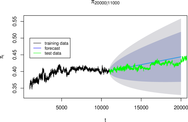
Figure 10 shows forecasts from this model along with training and test data.
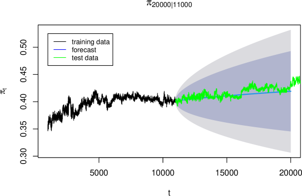
The forecasts extend much further into the future and follow the gradual upward trend more faithfully than the pure ARIMA model.
For comparison, we also fit an ARIMA model with drift:
##           ar1           ma1           ma2         drift
##  8.472755e-01 -1.396547e+00  4.324823e-01  4.695287e-06
The drift coefficient is small but positive. Over long horizons, this accumulates to produce an upward trend (Figure 11).
However, ARIMA with drift implies linear growth, which is theoretically inappropriate: must remain bounded in . The logarithmic regression model better respects this constraint.
8 Future work: incorporating covariates
Our forecasting models use only lagged values of to predict future confidentiality. This approach captures temporal patterns but ignores potential covariates that may affect adversary performance. Incorporating such covariates could improve forecast accuracy and provide insights into factors driving confidentiality degradation.
8.1 Information-theoretic covariates
The adversary learns from observing ciphers , but not all observations are equally informative. We could model the information content of each observation explicitly.
Define the information content of observation as
| (14) |
measured in bits. Observations with low probability under the adversary’s model carry more information.
Lagged values of could be used as predictors in a dynamic regression:
| (15) |
Alternatively, cumulative information (empirical entropy) could serve as a covariate. This would allow the model to adapt to the informativeness of recent queries, potentially tightening prediction intervals during periods of rapid learning.
8.2 Side-channel information
Beyond the cipher sequence, the adversary may obtain side-channel information. For example:
-
•
Timing information revealing query complexity
-
•
Access patterns indicating document relevance
-
•
External knowledge narrowing the plaintext space
Such events could be modeled as intervention variables or structural breaks. For instance, if the adversary learns that cipher maps to a subset , this constitutes an information gain equivalent to reducing the entropy of the plaintext distribution. Dynamic regression could incorporate indicator variables for such events, allowing the model to capture sudden jumps in adversary accuracy.
9 Conclusion
We have developed time series models to forecast confidentiality degradation in encrypted search systems under known-plaintext attacks. Our analysis demonstrates that standard ARIMA models can capture the temporal dynamics of adversary accuracy, while dynamic regression with logarithmic trend terms better incorporates domain knowledge about the theoretical behavior of learning curves.
9.1 Model comparison
The pure ARIMA model provides reasonable short-term forecasts and has the virtue of simplicity. However, it lacks theoretical grounding: ARIMA with drift predicts unbounded growth, eventually yielding impossible values ().
The logarithmic regression model () better reflects the expected learning dynamics. While it also lacks an asymptote (eventually predicting after approximately observations), this occurs far beyond any practical time horizon. The logarithmic form approximates the saturation behavior of adversary learning reasonably well over finite horizons.
9.2 Security policy implications
Consider a security threshold . Using our models, we estimate the critical time at which confidentiality falls below this threshold. Figure 12 shows as a function of .

For , we estimate , suggesting password reset should occur before 20,000 queries to maintain the threshold.
However, the 80% prediction intervals are substantially more conservative, sometimes recommending near-immediate password reset. This conservatism limits practical utility: overly frequent resets impose costs on users and administrators.
9.3 Limitations and future directions
The wide prediction intervals indicate substantial forecast uncertainty. This may stem from model misspecification or from genuine stochasticity in the adversary’s learning process. As discussed in Section 8, incorporating covariates (information content of queries, side-channel events) could reduce uncertainty and improve forecast accuracy.
9.3.0.1 The case for bounded models.
A fundamental limitation of ARIMA and logarithmic regression is that they do not respect the theoretical constraint . Both models eventually predict impossible values () at sufficiently long horizons. The correct theoretical form for adversary learning is a saturation model such as the exponential approach to asymptote:
| (16) |
where is the asymptotic accuracy (limited by model mismatch between adversary and true distribution), and control the initial value and convergence rate. This form captures three intuitive properties: the adversary starts with limited knowledge, improves rapidly at first, then approaches a ceiling as remaining words become difficult to distinguish.
Fitting such bounded models would require nonlinear estimation (e.g., nonlinear least squares) but would yield forecasts that remain theoretically valid at all horizons. We leave this extension to future work.
Despite these limitations, our analysis demonstrates that time series methods can provide quantitative guidance for encrypted search security policies, enabling data-driven decisions about system reinitialization timing.
9.4 Key insights for practitioners
Remark (Summary of Key Insights).
This analysis yields four actionable insights for practitioners deploying encrypted search systems:
-
1.
Entropy determines vulnerability: Lower-entropy plaintext distributions (predictable, repetitive queries) lead to faster confidentiality degradation. Encouraging query diversity slows adversary learning.
-
2.
High-frequency words fall first: The adversary correctly identifies common words before rare ones. If protecting high-value rare queries, confidentiality may remain acceptable longer than the aggregate measure suggests.
-
3.
Use conservative bounds: Prediction intervals are wide. For security policy, use the upper bound of the interval (pessimistic estimate) rather than the point forecast.
-
4.
Data-driven rotation: Given an organizational threshold , our models provide quantitative guidance for password rotation frequency, balancing security against operational costs.
References
- [1] (2006) Elements of information theory. 2nd edition, Wiley-Interscience, Hoboken, NJ. Cited by: ¶4.1.0.1, ¶4.1.0.1.
- [2] (1979) Distribution of the estimators for autoregressive time series with a unit root. Journal of the American Statistical Association 74 (366), pp. 427–431. Cited by: §7.1.
- [3] (2009) The elements of statistical learning: data mining, inference, and prediction. 2nd edition, Springer, New York. Cited by: §7.2.
- [4] (2012) Access pattern disclosure on searchable encryption: ramification, attack and mitigation. In Network and Distributed System Security Symposium (NDSS), Cited by: §2.
- [5] (2010-10) The ARIMAX model muddle. External Links: Link Cited by: §7.5.
- [6] (2000) Practical techniques for searches on encrypted data. In Proceedings 2000 IEEE Symposium on Security and Privacy. S&P 2000, pp. 44–55. Cited by: §2.
- [7] (1949) Human behavior and the principle of least effort. Addison-Wesley, Cambridge, MA. Cited by: ¶4.1.0.2.